Consortium

Introduction

Motivation

Particle dark matter, along with many ultraviolet scenarios, suggest that additional low-energy degrees of freedom remain to be discovered. In a basic scenario, bosonic fields on flat spacetime will form a perturbative effective field theory (EFT) \begin{equation}\label{EFTLag} \mathcal{L}=\Lag+\sum_{n=5}^{\infty}\sum_i\frac{\MAGG{n}{_i}\OperatorO{i}{n}}{\L^{n-4}},\end{equation} whose validity may be limited by the scale \(\L\). Where perturbation theory holds, it is exclusively the quadratic part of \(\Lag\) which determines the particle spectrum. The symmetries of this quadratic sector also dictate the non-linear structure, and may themselves receive non-linear corrections under the Noether procedure. No symmetric interactions may be excluded if the theory is to be stable against radiative corrections. Nonetheless, small symmetry-breaking parameters of the free theory inherit part of this radiative protection, and are technically natural.

The picture in \(\ \eqref{EFTLag}\ \) successfully describes all the fundamental bosons that are currently known to exist. The coordinate invariance of linearised gravity — as a symmetry — gives rise uniquely to non-linear general relativity and its predictive EFT extension; the Maxwell theory meanwhile gives rise to Yang–Mills. Small symmetry-breaking masses for both the vector gauge boson and graviton are technically natural, and are described by the Proca and Fierz–Pauli theories, respectively. Indeed, vector masses are actually observed in the weak sector, where the symmetry is restored by the Higgs mechanism.

Generalised Proca theory offers an alternative to the Higgs mechanism, and is an attractive dark sector candidate. Similarly, a small graviton mass is under investigation in cosmology; the non-linear completion in this case is dRGT gravity, which has intimate connections with generalised Proca theory.

Whilst \(\ \eqref{EFTLag}\ \) serves as a popular and conservative infrared foundation for the dark sector, it admits an uncomfortably large number of models. Even when restricting to bosonic fields without internal symmetries, the space of possibilities grows quickly with the field content. Once universal constraints on higher-spin fields have been imposed, the generalised Proca and dRGT theories will still be the lowest hanging fruits in an infinite tower of technically natural models. The fact that consistent interactions have not been found for most of these models does not exclude them from participating in the dark sector as an EFT, and we are in principle obliged to consider them.

An apparent danger of scaling up the field content in this way is the proliferation of parameters, which generally weaken predictivity. The point is that when properly calculated, the Occam penalty is sensitive only to the degree to which these parameters affect the observables. As an example, the presence of infinitely many parameters should not weaken perturbative quantum gravity: they are necessarily present once quantum mechanics is switched on, and give rise to universal low-energy predictions.

In practice, for most bosonic field configurations (excepting countably many special cases) even the unitary configurations of the free theory remain unknown, due to the sheer number of spin states that can be packaged into Lorentz tensors. By convenience of design, this specific problem is not apparent in many popular scenarios beyond the standard model, though it has long plagued extended theories of gravity. We are not aware of any physical reason why the dark sector should be restricted to simple field content, and a theory-agnostic approach which takes advantage of precision cosmology observables must confront this issue head-on.

Numerical polology

The formal algorithm for computing the free particle spectrum and associated unitarity of \(\ \eqref{EFTLag}\ \) has been known since the work of Van Nieuwenhuizen and Sezgin (Van Nieuwenhuizen 1973; Neville 1978, 1980; Sezgin 1981; Sezgin and Nieuwenhuizen 1980; Kuhfuss and Nitsch 1986; Karananas 2015, 2016; Mendonça and Schimidt Bittencourt 2020; Percacci and Sezgin 2020; Marzo 2022a, 2022b; Mikura, Naso, and Percacci 2023; Mikura and Percacci 2024), but the technique is computationally expensive. Computer algebra implementations have recently been developed (Lin, Hobson, and Lasenby 2019, 2020, 2021; Lin 2020; Barker, Marzo, and Rigouzzo 2024; Barker, Karananas, and Tu 2025), but these scale poorly with field complexity due to expression swell. For a scalable approach, the only avenue is numerical.

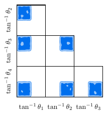
As a simple example, linear gravity is described by the Lichnerowicz theory in the metric perturbation \(\TensorField{_{\alpha\beta}}\), and this may be extended with a tuned Fierz–Pauli term to form the linearisation of massive gravity \begin{equation}\label{eq:FP}\begin{aligned} \Lag &= \Coupling{_1} \bigg[ \frac{1}{2} \PD{_\beta}\TensorField{} \PD{^\beta}\TensorField{} - \PD{^\alpha}\TensorField{_{\alpha\beta}} \PD{^\beta}\TensorField{} \\ &\quad - \frac{1}{2} \PD{_\gamma}\TensorField{^{\alpha\beta}} \PD{^\gamma}\TensorField{_{\alpha\beta}} + \PD{_\beta}\TensorField{^{\alpha\beta}} \PD{^\gamma}\TensorField{_{\alpha\gamma}} \bigg] \\ &\quad - \Coupling{_2} \bigg[ \TensorField{_{\alpha\beta}}\TensorField{^{\alpha\beta}} - \TensorField{}^2 \bigg]. \end{aligned}\end{equation} Since the theory parameters (collectively \(\Coupling{}\)) are a priori unconstrained, it is convenient to compactify the parameter space to a two-dimensional hypercube in \(\tan^{-1}\Coupling{}\). A posteriori, we know that the no-ghost and no-tachyon conditions following from \(\ \eqref{eq:FP}\ \) are \begin{equation}\label{eq:FP_unitarity} \Coupling{_1} < 0, \quad \Coupling{_2} > 0,\end{equation} and a numerical implementation of polology confirms this on the hypercube, as shown in Figure 1.

As a marginal extension of \(\ \eqref{eq:FP}\ \), we may consider the Fierz–Pauli–Proca theory, which adds a massive vector field \(\VectorField{_\alpha}\) through the Lagrangian \begin{equation}\label{eq:FPP}\begin{aligned} \Lag &= \Coupling{_3} \bigg[ -\frac{1}{2} \PD{_\alpha}\VectorField{_\beta} \PD{^\alpha}\VectorField{^\beta} + \frac{1}{2} \PD{_\alpha}\VectorField{^\alpha} \PD{_\beta}\VectorField{^\beta} \bigg] \\ &\quad - \frac{1}{2}\Coupling{_4} \VectorField{_\alpha}\VectorField{^\alpha}. \end{aligned}\end{equation} The combined unitarity conditions for \(\ \eqref{eq:FP}, \eqref{eq:FPP}\ \) are \begin{equation}\label{eq:FPP_unitarity} \Coupling{_1} < 0, \quad \Coupling{_2} > 0, \quad \Coupling{_3} > 0, \quad \Coupling{_4} < 0,\end{equation} and Figure 2 shows that these, too, are easy to find.

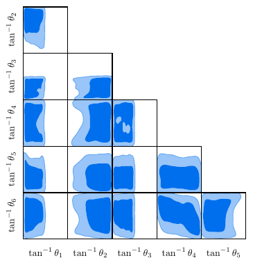
Whilst \(\ \eqref{eq:FP}, \eqref{eq:FPP}\ \) are well known models, we may use the same technique to study new theories, in which sectors are mixed. The most general Stueckelberg extension of massive gravity in which transverse diffeomorphism invariance is restored by the addition of an extra scalar \(\ScalarField\) is \begin{equation}\label{eq:TDiff}\begin{aligned} \Lag &= \frac{\Coupling{_1}}{2} \TensorField{_{\alpha\beta}}\TensorField{^{\alpha\beta}} + \Coupling{_5} \TensorField{}^2 + \Coupling{_6} \TensorField{} \PD{_\alpha}\VectorField{^\alpha} \\ &\quad - \Coupling{_6} \TensorField{} \PD{_\alpha}\PD{^\alpha}\ScalarField - \Coupling{_1} \PD{_\alpha}\VectorField{^\alpha} \PD{_\beta}\VectorField{^\beta} \\ &\quad + \Coupling{_1} \PD{_\beta}\VectorField{_\alpha} \PD{^\beta}\VectorField{^\alpha} + 2\Coupling{_1} \TensorField{^{\alpha\beta}} \PD{_\beta}\PD{_\alpha}\ScalarField \\ &\quad - 2\Coupling{_1} \TensorField{_{\alpha\beta}} \PD{^\beta}\VectorField{^\alpha} + \Coupling{_2} \PD{_\beta}\TensorField{} \PD{^\beta}\TensorField{} \\ &\quad + \Coupling{_3} \PD{_\alpha}\TensorField{^{\alpha\beta}} \PD{_\gamma}\TensorField{_\beta^\gamma} + \Coupling{_4} \PD{^\beta}\TensorField{} \PD{_\gamma}\TensorField{_\beta^\gamma} \\ &\quad - \frac{\Coupling{_3}}{2} \PD{_\gamma}\TensorField{_{\alpha\beta}} \PD{^\gamma}\TensorField{^{\alpha\beta}}. \end{aligned}\end{equation} The theory in \(\ \eqref{eq:TDiff}\ \) is parameterised by a six-dimensional hypercube: the numerical polology in Figure 3 reveals a sizeable unitary volume, containing an extra massive scalar of spin zero. Formally, the bounds of this region can be obtained by a straightforward but lengthy analysis, and are found to be \begin{equation}\label{eq:TDiff_unitarity} \begin{gathered} \Coupling{_1} < 0, \quad \Coupling{_3} < 0, \quad \Coupling{_5} < \frac{-\Coupling{_1}^2 + \Coupling{_1}\Coupling{_6} - \Coupling{_6}^2}{6\Coupling{_1}}, \\ \Coupling{_2} > \frac{2\Coupling{_1}^2\Coupling{_3} - 2\Coupling{_1}\Coupling{_3}\Coupling{_6} - 6\Coupling{_1}\Coupling{_4}\Coupling{_6} - \Coupling{_3}\Coupling{_6}^2}{12\Coupling{_1}^2}. \end{gathered}\end{equation} For cosmological phenomenology, only the renormalised values of the \(\Coupling{}\) are interesting. The point is that a well-explored unitary posterior of these \(\Coupling{}\) is overwhelmingly cheaper to obtain, as compared to rejection-sampling dependant on formal conditions such as in \(\ \eqref{eq:TDiff_unitarity}\ \).

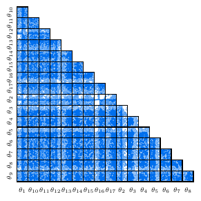
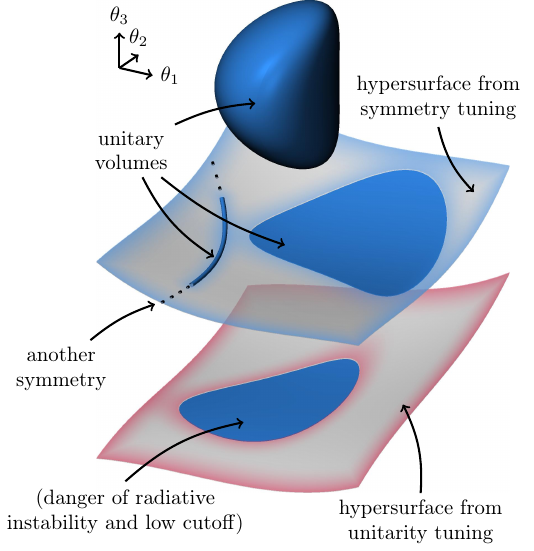
The theory in \(\ \eqref{eq:TDiff}\ \) is inflated with spurions, but for genuine gauge symmetries the concept of unitary volumes is also critical. In general, the parameter space will not contain volumes, but rather unitary hypersurfaces of lower codimension: only when these hypersurfaces are associated with the emergence of new gauge symmetries are they expected to be stable against radiative corrections. Modern sampling techniques happen to be well-suited to finding such features. To illustrate this, we consider the completely general parity-preserving tensor–vector–scalar theory, \[\begin{aligned} \Lag &= \Coupling{_1} \VectorField{_\alpha}\VectorField{^\alpha} + \Coupling{_2} \TensorField{_{\alpha\beta}}\TensorField{^{\alpha\beta}} + \Coupling{_3} \TensorField{}^2 \nonumber\\ &\quad + \Coupling{_4} \TensorField{}\ScalarField + \Coupling{_5} \ScalarField^2 + \Coupling{_6} \TensorField{} \PD{_\alpha}\VectorField{^\alpha} \nonumber\\ &\quad + \Coupling{_7} \ScalarField \PD{_\alpha}\VectorField{^\alpha} + \Coupling{_8} \PD{_\alpha}\VectorField{^\alpha} \PD{_\beta}\VectorField{^\beta} \nonumber\\ &\quad + \Coupling{_9} \TensorField{^{\alpha\beta}} \PD{_\beta}\PD{_\alpha}\ScalarField + \Coupling{_{10}} \TensorField{} \PD{_\alpha}\PD{^\alpha}\ScalarField \nonumber\\ &\quad + \Coupling{_{11}} \TensorField{_{\alpha\beta}} \PD{^\beta}\VectorField{^\alpha} + \Coupling{_{12}} \PD{_\beta}\VectorField{_\alpha} \PD{^\beta}\VectorField{^\alpha} \nonumber\\ &\quad + \Coupling{_{13}} \PD{_\beta}\TensorField{} \PD{^\beta}\TensorField{} + \Coupling{_{14}} \PD{_\alpha}\TensorField{^{\alpha\beta}} \PD{_\gamma}\TensorField{_\beta^\gamma} \nonumber\\ &\quad + \Coupling{_{15}} \PD{^\beta}\TensorField{} \PD{_\gamma}\TensorField{_\beta^\gamma} + \Coupling{_{16}} \PD{_\gamma}\TensorField{_{\alpha\beta}} \PD{^\gamma}\TensorField{^{\alpha\beta}} \nonumber\\ &\quad + \Coupling{_{17}} \PD{_\alpha}\ScalarField \PD{^\alpha}\ScalarField, \label{eq:SVT} \end{aligned}\] which has 17 free parameters. The bulk of the parameter space is sick, but by treating unitarity violation as a likelihood penalty we are naturally driven to the healthy features, as shown in Figure 4.

Implementation

Massive unitarity

Focussing on the sector of spin \(J\) and parity \(P\), the wave operator in a basis of spin projection operators is denoted \(\WaveOperatorJP{J}{P}\), where \(k\equiv\sqrt{\tensor{k}{_\alpha} \tensor{k}{^\alpha}}\) is the momentum. For general \(k\), this admits a collection of null eigenvectors \(\WaveOperatorJP{J}{P}\cdot\NullVector{J}{P}{a} = 0\) which encode all the gauge symmetries acting on the \(J^P\) sector. Once the \(\theta\) are sampled, these symmetries may be computed numerically from a polynomial expansion \begin{equation}\label{eq:PolyExpansions}\begin{aligned} \WaveOperatorJP{J}{P} &= \sum_{n} \WaveOperatorJPn{J}{P}{n} k^n, \\ \NullVector{J}{P}{a} &= \sum_{n} \NullVectorN{J}{P}{a}{n} k^n, \end{aligned}\end{equation} which gives rise to a block singular value decomposition problem. The gauge-regularised wave operator \begin{equation}\label{eq:RegularizedWaveOperator} \RegWaveOperatorJP{J}{P} \equiv \WaveOperatorJP{J}{P} + \sum_a \NullVector{J}{P}{a} \cdot \NullVectorConj{J}{P}{a},\end{equation} then defines a polynomial eigenvalue problem in \(k\), which yields a candidate spectrum of masses \(k^2=m(\Coupling{})^2\). Because the construction in \(\ \eqref{eq:PolyExpansions}\ \) does not give rise to normalised \(\NullVector{J}{P}{a}\), this spectrum will generally be polluted by spurious ‘gauge’ masses, though these are readily stripped by comparing their null eigenvectors with the gauge sector of the kernel. The physical masses \(m(\Coupling{})\) are associated with null eigenvectors \(\RegWaveOperatorJPm{J}{P} \cdot \PhysNullVector{J}{P}{s} = 0\), for which the condition \begin{equation}\label{eq:NoTachyon} m(\Coupling{})^2 > 0,\end{equation} is the usual no-tachyon criterion.

A viable no-ghost criterion is known from (Barker, Marzo, and Rigouzzo 2024) to be \begin{equation}\label{eq:MassiveNoGhost} \NewRes{k^2}{m(\Coupling{})^2}\left(P\,{\rm tr}\,\MoorePenroseJP{J}{P}\right) > 0,\end{equation} where \(\MoorePenroseJP{J}{P}\) is the Moore–Penrose pseudoinverse of \(\WaveOperatorJP{J}{P}\). Even with sampled \(\Coupling{}\), obtaining the pseudoinverse remains a symbolic problem. For a numerical alternative, we consider the matrix \(\GaugeMatrixJP{J}{P}\) whose columns are the \(\NullVectorm{J}{P}{a}\), and which defines the non-gauge projection \begin{equation}\label{eq:GaugeProjection}\begin{aligned} &\ProjNullVector{J}{P}{s} \equiv \\ &\qquad \left[ \mathsf{1} - \GaugeMatrixJP{J}{P} \left( \GaugeMatrixJPConj{J}{P} \GaugeMatrixJP{J}{P} \right)^{-1} \GaugeMatrixJPConj{J}{P} \right] \cdot \PhysNullVector{J}{P}{s}, \end{aligned}\end{equation} of the massive null eigenvectors. The no-ghost condition in \(\ \eqref{eq:MassiveNoGhost}\ \) is then equivalent to \begin{equation}\label{eq:NoGhost} P \, \ProjNullVectorConj{J}{P}{s} \cdot \biggl( \sum_{n} n \, \WaveOperatorJPn{J}{P}{n} m(\Coupling{})^{n-1} \biggr) \cdot \ProjNullVector{J}{P}{s} > 0,\end{equation} by a Kato expansion.

Mass dimensions

So far, the mass dimensions of the \(\Coupling{}\) have not been specified. Indeed, the fields themselves only acquire a definite canonical dimensions once the spectrum has been computed, and the same must be true of the \(\Coupling{}\). Let \([\Coupling{_i}]=\Dimension{_i}\), whilst we know \([k]=[m(\Coupling{})]=1\). We have access numerically to the \(m(\Coupling{})\), and a rescaling of the mass unit yields \begin{equation}\label{eq:MassRescaling} \sum_{i} \Dimension{_i} \, \frac{\partial\ln m(\Coupling{})}{\partial \ln \Coupling{_i}} = 1.\end{equation} Any choice of \(\Dimension{_i}\) that satisfies \(\ \eqref{eq:MassRescaling}\ \) for all \(m(\Coupling{})\) is valid. To ensure that the Lagrangian density has the correct mass dimension, under the usual convention that propagating bosons have mass dimension one, we seek integer solutions and fix \(\min_i \Dimension{_i} = 0\).

Softly-broken symmetries

At some fixed reference scale \(\KRef{}\), each \(\WaveOperatorJPRef{J}{P}\) will have a family of non-zero real eigenvalues \(\RefEig{J}{P}{s}\), besides any vanishing eigenvalues corresponding to gauge symmetries \(\NullVectorRef{J}{P}{a}\) which are present in the underlying theory. Working from a given sample \(\Coupling{}\), the \(\RefEig{J}{P}{s}\) may be ‘walked down’ in \(\Coupling{}\)-space via a process of steepest descent, driven by the Hellmann–Feynman theorem \begin{equation}\label{eq:HellmannFeynman} \begin{aligned} \frac{\partial \RefEig{J}{P}{s}}{\partial \Coupling{_i}} &= \\ &\!\!\!\!\!\! \EigVectorRefConj{J}{P}{s} \cdot \frac{\partial \WaveOperatorJPRef{J}{P}}{\partial \Coupling{_i}} \cdot \EigVectorRef{J}{P}{s}, \end{aligned}\end{equation} where \(\EigVectorRef{J}{P}{s}\) is the eigenvector of the corresponding \(\RefEig{J}{P}{s}\). Such trajectories are classified by examining the physical mass spectrum at their termini. Eigenvalues corresponding to propagating sectors always terminate at \({m(\Coupling{})\to\KRef{}}\). Meanwhile, the smooth disappearance of one or more \(m(\Coupling{})\to 0\) signals the emergence of a softly-broken gauge symmetry \(\NullVectorSoft{J}{P}{a}\) which may be reconstructed from \(\ \eqref{eq:PolyExpansions}\ \) by considering a range of \(\KRef{}\).

If all the \(m(\Coupling{})\) can be removed by flowing samples from a unitary sub-volume to bordering surfaces of lower codimension, then the unitary volume defines a technically natural theory.

The radiative corrections to the mass spectrum of a technically natural theory may be estimated by a spurion analysis. A parameter which softly breaks a symmetry is identified by the function \begin{equation}\label{eq:SpurionCondition} \tensoraliased{\Theta}{^{{a}_{{J}^{{P}}}}_{{i}}} \equiv \Theta\left[ \NullVectorSoft{J}{P}{a}\cdot \frac{\partial \WaveOperatorJP{J}{P}}{\partial \Coupling{_i}} \cdot \NullVectorSoft{J}{P}{a} \right].\end{equation} Assuming interactions to give rise to the cutoff \(\Lambda\), and working at the renormalisation scale \(\mu\), the one-loop corrections are then expected to be \begin{equation}\label{eq:RadiativeCorrections} \delta\Coupling{_i}\sim\frac{1}{16\pi^2}\log\left(\frac{\Lambda}{\mu}\right) \sum_{j,{a}_{{J}^{{P}}}} \tensoraliased{\Theta}{^{{a}_{{J}^{{P}}}}_{{i}}} \tensoraliased{\Theta}{^{{a}_{{J}^{{P}}}}_{{j}}} \tensoraliased{c}{^j_i} \Coupling{_j}^{\tensoraliased{d}{^j_i}},\end{equation} where the \(c^j_i\) are dimensionless coefficients of order unity, and we filter only for positive integer powers with \begin{equation}\label{eq:DimensionFilter} \tensoraliased{d}{^j_i}\equiv \begin{cases} \Dimension{_i}/\Dimension{_j} & \Dimension{_j} | \Dimension{_i}, \\ -\infty & \text{otherwise}. \end{cases}\end{equation}

Sampling

The criteria in \(\ \eqref{eq:NoTachyon}, \eqref{eq:NoGhost}\ \) may thus be reached entirely by numerical linear algebra operations, once the \(\Coupling{}\) is sampled. An initial, light per-theory application of computer algebra is required only to extract the symbolic \(\WaveOperatorJPn{J}{P}{n}\), and this problem was previously solved for any theory by the Wolfram Language implementation in (Barker, Marzo, and Rigouzzo 2024; Barker, Karananas, and Tu 2025).

Given the \(\WaveOperatorJPn{J}{P}{n}\) matrices, the Julia language is a naturally performant choice for numerical polology; a sampler explores the compactified \(\Coupling{}\) hypercube, and an evaluator uses optimal BLAS/LAPACK routines to probe the spectrum at each point.

The central importance of sampling allows a natural connection to established precision cosmology workflows. The unitary posterior may be exported in the standard GetDist format, as visualised in Figure 1, Figure 2, Figure 3, Figure 4. These posteriors may be ingested by pipelines which probe any other phenomenology sensitive to the free \(\Coupling{}\); we will see presently that a wealth of such probes are already in mainstream use, and that for the most part they are needlessly restricted to simple field content.

Sampling, by itself, admits many variants. For the current implementation, we use a nested sampler with a likelihood \(\mathcal{L} = \prod_{m(\Coupling{})} u_{m(\Coupling{})}\), where \begin{equation}\label{eq:SoftLikelihood} u_{m(\Coupling{})} \equiv \begin{cases} 1 & U_{m(\Coupling{})} > 0, \\ e^{\l U_{m(\Coupling{})}} & U_{m(\Coupling{})} \leq 0, \end{cases}\end{equation} and the \(U_{m(\Coupling{})}\) correspond — across all \(m(\Coupling{})\) — to the left hand side of the inequalities in \(\ \eqref{eq:NoTachyon}, \eqref{eq:NoGhost}\ \). The penalty for unitarity violation is set by the scale \(\lambda\).

Unitarity, computed in this way, is exceptionally lean; the compiled evaluator has a millisecond runtime, three orders of magnitude faster than modern Boltzmann solvers. This is to be compared to symbolic computation, which can take many hours when parallelised on a cluster. In turn, this economy facilitates the large \(n_{\text{live}}{}\sim 10^4\) used in Figure 1, Figure 2, Figure 3, Figure 4, which is necessary in practice to resolve the fine structures associated with particle physics requirements — by contrast, phenomenological constraints on cosmological parameters are often smoother, and more amenable to kernel density estimation.

The unitarity evaluator is also extensible to a more comprehensive science stack; current by-products include the gauge symmetries and particle masses, but explicit cutoffs can also be computed.

Astroparticle physics

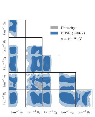
The derived quantities associated with the science stack admit various phenomenological constraints, which can be applied as multiplicative weights to the unitary posterior. We demonstrate this using four independent probes, applied to the theory in \(\ \eqref{eq:TDiff}\ \). For all probes, we exploit derived masses. This requires us to specify a reference scale, i.e. a unit in which the \(\Coupling{}\) of nonzero mass dimension is measured: we denote this scale as \(\mu\) by loose analogy with the renormalisation scale.

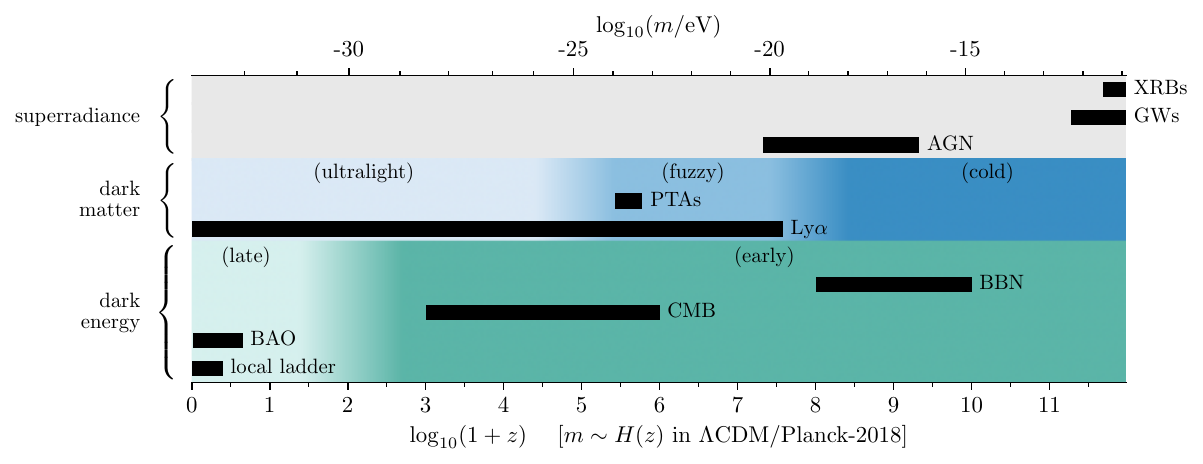
Phenomenologically, attention is drawn to mass scales which maximally affect the observables. Figure 5 shows these scales to be very low in astrophysics and cosmology, at \(m\ll1\,\text{eV}\). Such light particles sometimes are sometimes well-motivated, as in the case of the Peccei–Quinn mechanism which underpins the QCD axion. In the theory-agnostic approach, however, this pressure for light species gives rise to precisely the naturalness problem which numerical polology is designed to address. The most desirable mass scale depends on the observational domain, and on the specific problem that the theory is intended to solve.

Superradiance

Ultralight bosons trigger superradiant instabilities of spinning black holes (BHs), so BH observations exclude boson masses within a corresponding window (Arvanitaki, Baryakhtar, and Huang 2015). In its basic form, superradiance is sensitive only to the Lagrangian, but is agnostic with respect to the dynamical configuration of the fields. This advantage is not shared by the cosmological probes below, which rely on extended models. Constraints arise for any BH whose horizon is comparable to the Compton wavelength of the boson. Heavy species are constrained by X-ray binaries (XRBs) and gravitational wave (GW) events; light species by active galactic nuclei (AGN). The BH spin, and thus the quality of the constraint, depends strongly on the population from which the BH is drawn. Beyond the free mass, superradiant instability is additionally sensitive to the boson spin, and to self-interactions. A thorough superradiance implementation will thus be able to take advantage of the full tower of derived parameters in numerical polology. This becomes useful if, for example, an improved understanding of BH demography reveals gaps that cannot be explained by astrophysical processes alone.

We use precomputed exclusion tables for M33 X-7 (Orosz et al. 2007), a stellar-mass XRB probing \(m\sim 10^{-13}\text{--}10^{-11}\,\text{eV}\). The survival probability provides a smooth weight in \([0,1]\) for the \(0^+\) scalar mass. As shown in Figure 6 (left), superradiance excludes \(63.8\%\) of the unitary posterior, carving characteristic exclusion bands from the coupling space.

Dark matter

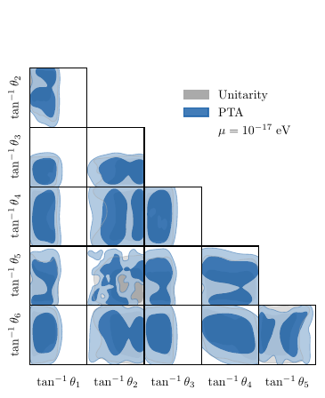
Bosons that account for a significant fraction of ultralight dark matter (ULDM) impose a cutoff in the matter power spectrum and suppress structure formation on small scales. The Ly forest provides the strongest constraint of \(m\gtrsim 2\times 10^{-20}\,\text{eV}\) for scalar ULDM (Rogers and Peiris 2021). Coincidentally, coherent oscillations of bosons whose masses are near to this bound would also give rise to correlated residuals in pulsar timing arrays (PTAs) (Smarra et al. 2023). Constraints from small-scale structure and pulsar timing vary widely according to the abundance fraction and local density of the ULDM, which must additionally be tied to a convincing production mechanism.

To illustrate how the ULDM scenario augments the basic theory with extra model parameters, we note that PTAs can also be sensitive to quasiparticle fluctuations in virialised ULDM halos, corresponding to boson masses far above the Ly bound and typical PTA sensitivity window (Kim and Mitridate 2024). The NANOGrav 12.5-year dataset places an upper bound on the local dark matter density as a function of the scalar mass, with peak sensitivity at \(m\sim 10^{-17}\,\text{eV}\). Assuming a local overdensity of \(\rho/\rho_0 = 5\times 10^4\), the PTA constraint excludes \(95.8\%\) of the posterior, as shown in Figure 6 (right). At the standard local density (\(\rho = \rho_0\)), current PTA data does not exclude any masses.

Dark energy

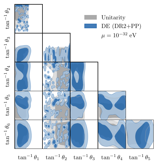
In the canonical quintessence scenario, a massive scalar field has an effective equation of state that transitions from \(w\approx -1\) to \(w \approx 0\) at the epoch \(m\sim H(z)\) (Turner 1983; Marsh 2016). Variations on this theme are known to strongly affect the Hubble tension via early dark energy models, and may be useful in response to recent signals for dynamical dark energy at late times. Such effects can, in principle, be constrained even through to Big Bang nucleosynthesis (BBN), beyond which the expansion history becomes speculative. As with ULDM, applications of light bosons to dark energy require extended models with tuned initial conditions.

Focussing on dynamical dark energy in the late Universe, we use the DESI DR2 BAO measurements (Abdul Karim et al. 2025) combined with Pantheon\(+\)SH0ES supernovae (Scolnic et al. 2022), marginalising over \(\Omega_m\) and \(H_0 r_d\). The resulting constraint on the \(0^+\) scalar mass, shown in Figure 7, excludes \(90.7\%\) of the unitary posterior. This probes an entirely different mass window (\(m\sim 10^{-33}\,\text{eV}\), comparable to \(H_0\)) from the astrophysical constraints above.

Graviton dispersion

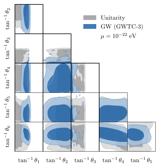
A massive graviton modifies the dispersion relation of gravitational waves, causing frequency-dependent propagation speeds that are detectable in compact binary coalescence signals (Abbott et al. 2025). The GWTC-3 combined analysis of 43 binary BH events yields the bound \(m_g \leq 2.42\times 10^{-23}\,\text{eV}\) at \(90\%\) credibility, surpassing the Solar System ephemeris bound of \(3.16\times 10^{-23}\,\text{eV}\) (Bernus et al. 2020). Unlike the scalar probes above, this constrains the \(2^+\) graviton mass. As shown in Figure 8, the GWTC-3 bound excludes \(20.1\%\) of the posterior.

These constraints are composable: since each acts as an independent multiplicative weight, they can be applied sequentially to produce joint posteriors combining unitarity with any subset of observational probes.

Extensions

The functionality shown above is illustrative, and many extensions are possible.

The high dimensionality of the \(\Coupling{}\)-space, and convoluted shape of the physically significant regions, are well suited to nested sampling. Unitary volumes are currently represented by likelihood plateaus, which are known to be difficult for samplers to explore. In all cases, it is the boundary of lower-codimension features which are of physical interest (see Figure 9). Unitary volumes are defined by such boundaries (so long as one picks the correct side) much like emergent gauge symmetries. This understanding shifts the focus to developing more sophisticated likelihood penalties for unitarity violation.

An associated problem is the lack of a physical measure on the \(\Coupling{}\) hypercube. It is interesting to consider whether the derived quantities, such as masses, can help to define such a measure. The \(\Coupling{}\) parameterisation is also arbitrary, and follows from the conventions in (Barker, Marzo, and Rigouzzo 2024; Barker, Karananas, and Tu 2025). A more natural parameterisation factors out mass dimensions, with parameters of common dimension spanning hyperspheres. Moreover, the full processing of a given model is hierarchical: gauge hypersurfaces, where identified in a parent theory, give rise to constrained models, and so on. These models are numerically discovered and numerically defined, which is a property that the original parameterisation does not share. It becomes necessary to either reverse-engineer the constraint (for example, via symbolic regression), or to soften the physical properties of the science stack in a way that remains stable as child-theories are discovered at increasing depth.

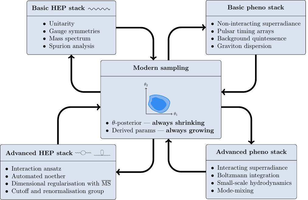
By design, the phenomenological plugins are arbitrarily extensible (see Figure 10). Here, we have illustrated the ‘low-hanging fruit’ of mass exclusions. These serve to constrain the model, but they do not help us to alleviate tensions. For the pipeline to be used in this way, the derived quantities must lead to large scale structure and microwave background predictions which require per-parameter inference.

Extensions to the science stack are intended to work in tandem with phenomenological constraints. It is expected that relevant theories will provide new, light species of interest in cosmology. An extended stack will constrain the interactions so as to suitably reduce quantum corrections to this stack. Constrained interactions will then feed back into the phenomenology, and so on.

There are two less ambitious extensions to the science stack. Firstly, the inclusion of the massless sector has so-far been worked out only analytically: a numerical implementation is obviously necessary, since new massless degrees of freedom are probably unacceptable. Secondly, we note that extension to fermionic fields is straightforward, though tedious, and that the same is probably true for simple internal symmetries.