Software and computational tools
All my software is dual-hosted on GitHub and GitLab.
Below are my main projects with live repository information pulled from GitHub.

![]()
![]()
![]()
![]()
![]()
![]()
![]()
![]()
![]()
![]()
![]()
![]()
![]()
PSALTer: Particle Spectrum for Any Tensor Lagrangian
Version 2.0.2
- Updated logos.
- Updated
README.md.
License
Copyright © 2022 Will Barker, Giorgos Karananas, Carlo Marzo, Claire Rigouzzo and Haochen Tu.
PSALTer is distributed as free software under the GNU General Public License (GPL).
PSALTer is provided without warranty, or the implied warranty of merchantibility or fitness for a particular purpose.
If PSALTer was useful to your research, please cite us using the following BibTeX:
@article{Barker:2024juc,
    author = "Barker, Will and Marzo, Carlo and Rigouzzo, Claire",
    title = "{PSALTer: Particle Spectrum for Any Tensor Lagrangian}",
    eprint = "2406.09500",
    archivePrefix = "arXiv",
    primaryClass = "hep-th",
    month = "6",
    year = "2024"
}
@article{Barker:2025qmw,
    author = "Barker, Will and Karananas, Georgios K. and Tu, Haochen",
    title = "{The particle spectra of parity-violating theories: A less radical approach and an upgrade of PSALTer}",
    eprint = "2506.02111",
    archivePrefix = "arXiv",
    primaryClass = "hep-th",
    month = "6",
    year = "2025"
}
About
PSALTer is a software package for Wolfram (formerly Mathematica) designed to predict the propagating quantum particle states in any tensorial field theory, including (but not limited to) just about any theory of gravity. The free action $S_{\text{F}}$ must have the structure
S_{\text{F}}=\int\mathrm{d}^4x\ \zeta(x)^{\text{T}}\cdot\Big[\mathcal{O}(\partial)\cdot\zeta(x)-j(x)\Big],
where the ingredients are:
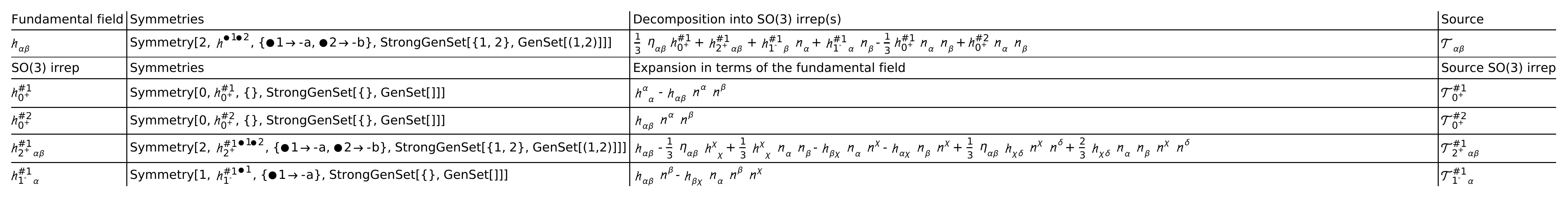
- The dynamical fields $\zeta(x)$ are real tensors, which may be a collection of distinct fields, each field having some collection of spacetime indices ($\mu$, $\nu$, etc.), perhaps with some symmetry among the indices.
- The wave operator $\mathcal{O}(\partial)$ is a real, second-order differential operator constructed from the flat-space metric $\eta_{\mu\nu}$, partial derivative $\partial_\mu$ and totally antisymmetric $\epsilon^{\mu\nu\sigma\lambda}$ tensor, linearly parameterised by a collection of coupling coefficients. Note that Ostrogradsky’s theorem discourages higher-derivative operators, but even if it did not we note that the apparent order may always be lowered by the introduction of extra fields.
- The source currents $j(x)$ are conjugate to the fields $\zeta(x)$. They encode all external interactions to second order in fields, whilst keeping the external dynamics completely anonymous.
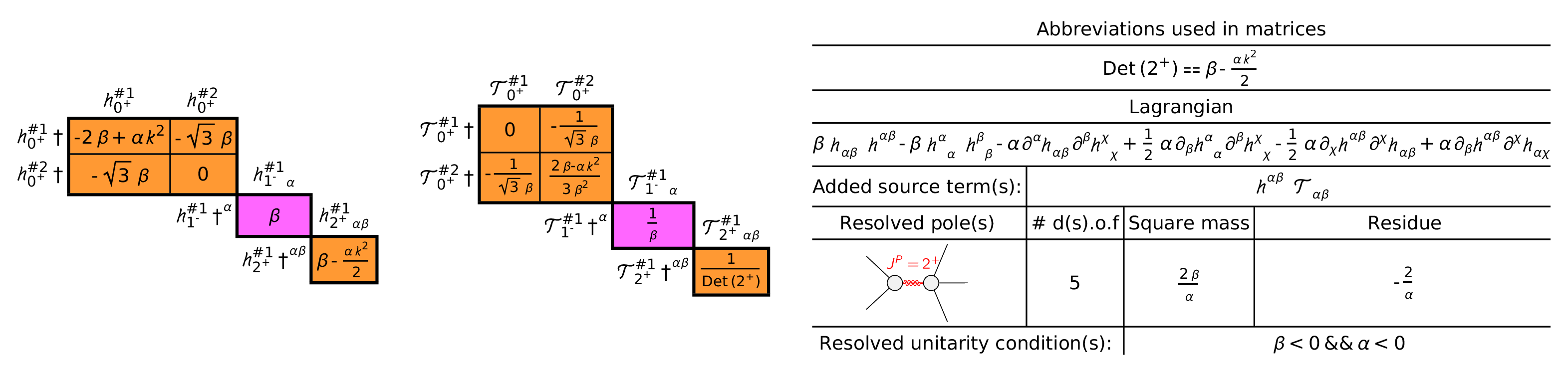
Example: massive gravity
As a demonstration, we consider the Fierz-Pauli linearised massive gravity theory
S=\int\mathrm{d}^4x\ \Big[\alpha\big(-\partial^\mu h_{\mu\nu}\partial^\nu h+\tfrac{1}{2}\partial_\mu h\partial^\mu h-\tfrac{1}{2}\partial_\sigma h^{\mu\nu}\partial_\sigma h_{\mu\nu}+\partial_\nu h^{\mu\nu}\partial^\sigma h_{\mu\sigma}\big)+\beta\big(h^{\mu\nu}h_{\mu\nu}-h^2\big)+h^{\mu\nu}T_{\mu\nu}\Big],
where $\alpha$ and $\beta$ are coupling coefficients, $h_{\mu\nu}$ is the metric perturbation with trace $h\equiv h_{\mu}^{\mu}$, and $T^{\mu\nu}$ is the linearised stress-energy tensor of matter, which is the source conjugate to $h_{\mu\nu}$.
In a fresh notebook we first load the package:
<<xAct`PSALTer`;
Next, we define Lagrangian couplings $\alpha$ and $\beta$ as Coupling1 and Coupling2 using the command DefConstantSymbol from xAct:
DefConstantSymbol[Coupling1,PrintAs->"\[Alpha]"];
DefConstantSymbol[Coupling2,PrintAs->"\[Beta]"];
Next, we use the command DefField from PSALTer to define the metric perturbation $h_{\mu\nu}$ as the symmetric, rank-two tensor field MetricPerturbation:
DefField[
    MetricPerturbation[-a,-b],
    Symmetric[{-a,-b}],
    PrintAs->"\[ScriptH]",
    PrintSourceAs->"\[ScriptCapitalT]"
];
The output should look like:
To compute the spectrum, we plug the Lagrangian into the ParticleSpectrum function from PSALTer:
ParticleSpectrum[
    Coupling1*(
	(1/2)*CD[-b]@MetricPerturbation[a,-a]*CD[b]@MetricPerturbation[c,-c]
	-CD[a]@MetricPerturbation[-a,-b]*CD[b]@MetricPerturbation[c,-c]
	-(1/2)*CD[-c]@MetricPerturbation[a,b]*CD[c]@MetricPerturbation[-a,-b]
	+CD[-b]@MetricPerturbation[a,b]*CD[c]@MetricPerturbation[-a,-c]
    )
    +Coupling2*(
        MetricPerturbation[-a,-b]*MetricPerturbation[a,b]
        -MetricPerturbation[a,-a]*MetricPerturbation[b,-b]
    ),
    TheoryName->"MassiveGravity",
    MaxLaurentDepth->3
];
The output should look like:
Documentation
The package includes a notebook with the basic example above. This notebook will try to save PDF graphics files to the directory in which it is saved, so it is better not to run it from within your actual installation. For instance, to copy the file to your home directory and run it there using the front end (notebook), you can use: ```console, bash [user@system PSALTer]$ cp xAct/PSALTer/Documentation/English/Examples.nb ~/Examples.nb [user@system PSALTer]$ cd [user@system English]$ wolframnb Examples.nb &
The theory underlying the package is developed across two papers:
- [The first paper](https://arxiv.org/abs/2406.09500) presents _PSALTer_ v 1.0.0 (basic functionality).
- [The second paper](https://arxiv.org/abs/2503.#####) presents _PSALTer_ v 2.0.0 (extension to parity violation and breaking changes).

## General use

### Pre-defined geometry

When you first run `` <<xAct`PSALTer` `` the software defines a Minkowski manifold with the ingredients:

| _Wolfram Language_      | Output format                            | Meaning                      |
|-------------------------|------------------------------------------|------------------------------|
| `a`, `b`, `c`, ..., `z` | $\alpha$, $\beta$, $\gamma$, ... $\zeta$ | Cartesian coordinate indices |
| `G[-m,-n]`              | $\eta_{\mu\nu}$                          | Minkowski metric             |
| `CD[-m]@`               | $\partial_{\mu}$                         | Partial derivative           |
| `epsilonG[-m,-n,-s,-l]` | $\epsilon_{\mu\nu\sigma\lambda}$         | Totally antisymmetric tensor |

For those familiar with _xAct_, note that calls to `DefManifold` and `DefMetric` are made internally at this stage. The minimal workflow in _PSALTer_ is to compute spectra based on a free Lagrangian density which has already been worked out, and simply needs to be plugged into the `ParticleSpectrum` function once the relevant fields are defined using `DefField` and the relevant coupling constants are defined using `DefConstantSymbol`. A more advanced workflow uses the geometric environment of _PSALTer_ and various tools from _xAct_ to first compute the free Lagrangian density by _linearising_ some other model. In the latter case, it is important to first understand more about the geometric environment of _PSALTer_, which is established internally by the following calls:
```mathematica
DefManifold[M4,4,IndexRange[{a,z}]];
DefMetric[-1,G[-a,-c],CD,{",","\[PartialD]"},PrintAs->"\[Eta]",FlatMetric->True,SymCovDQ->True];
In particular, the flat metric environment can be inconvenient when the model to be linearised is gravitational in nature, relying on some curvature tensor. At the practical level, one can always obtain the correct linearisation by reinterpreting the model as a field theory on flat spacetime: this approach is guaranteed to work because particle physics is not actually sensitive to geometry per se. Alternatively, one can prepare the linearised expression in a separate xAct session, taking advantage of the full geometric interpretation, and then copy the resulting Wolfram Language expression directly into the PSALTer session. Care must be taken in this case to ensure that the indices are correctly matched.
Function DefField
DefField[<Fld>[]]
defines a scalar field <Fld> and exports the field kinematics to a PDF file.
DefField[<Fld>[<Ind1>,<Ind2>,...]]
defines a tensor field <Fld> with indices <Ind1>, <Ind2>, etc., and exports the field kinematics to a PDF file.
DefField[<Fld>[<Ind1>,<Ind2>,...],<Symm>]
defines a tensor field <Fld> with indices <Ind1>, <Ind2>, etc. and symmetry <Symm>, and exports the field kinematics to a PDF file.
Details and options
- The syntax of
DefFieldis almost identical to that ofDefTensorin xTensor. - Up to three comma-separated indices may be drawn from the contravariant
a,b,c, up toz, the covariant-a,-b,-c, up to-z, or any admixture. - It is strongly recommended to use clear, alphanumeric names for
<Fld>, because the name of the field kinematics file will beFieldKinematics<Fld>.pdf. As explained below, thePrintAsoption allows the user to specify the symbol used for formatting the field in the front end (notebook) and the exported PDFs. - The symmetry
<Symm>can be one of the following, where<SymmInd1>,<SymmInd2>, etc. are any two or three fully covariant or contravariant, comma-separated indices drawn verbatim from<Ind1>,<Ind2>, etc.:Symmetric[{<SymmInd1>,<SymInd2>,...}]denotes symmetrized indices.Antisymmetric[{<SymmInd1>,<SymInd2>,...}]denotes antisymmetrized indices.
- In the front end (notebook) the currently-evaluating subroutine is displayed temporarily.
- In the terminal, the currently-evaluating subroutine is sent to
STDOUT. - Whilst
DefFieldprints a preview of the field kinematics in the front end (notebook) it always returnsNull. - The following options may be given:
PrintAsis the symbol that<Fld>will use for formatting. In the front end (notebook), symbols can be entered directly. Programmatically, the Wolfram Language admits named characters such as"\[<Name>]". The default is $\zeta$ or"\[Zeta]".PrintSourceAsis the symbol that the source conjugate to<Fld>will use for formatting. The syntax is identical toPrintAs. The default is $j$ or"\[ScriptJ]".
Function ParticleSpectrum
ParticleSpectrum[<Lagr>];
computes the spectrum of the Lagrangian <Lagr>, and exports a spectrograph to a PDF file.
Details and options
- The Lagrangian
<Lagr>must be a valid, linearised Lagrangian density. The expression must be a Lorentz-scalar. Each term must be quadratic in field(s) which have already been defined usingDefField. Each term must be linear in coupling constant(s) which have already been defined usingDefConstantSymbolfrom xTensor. Other allowed ingredients areCD,GandepsilonG. Do not try to include the term coupling the fields to their conjugate sources: this is accounted for internally. - In the front end (notebook) the currently-evaluating subroutine is displayed temporarily.
- In the terminal, the currently-evaluating subroutine is sent to
STDOUT. - Whilst
ParticleSpectrumprints a preview of the spectrograph in the front end (notebook) it always returnsNull. - The following options may be given:
TheoryNameis a mandatory option and must be set to an alphanumeric string"<ThrNme>". The name of the spectrograph file will beParticleSpectrograph<ThrNme>.pdf.Neglectmust be a list of the form{{<Spn1>,<Pty1>},{<Spn2>,<Pty2>},...}, enumerating the spins and parities of the sectors which are to be neglected in the analysis, where<Spn1>and<Spn2>etc. are0,1,2or3and<Pty1>,<Pty2>etc. are1or-1. The massless spectrum will not be computed if any sectors have been neglected. The default is{}.MasslessSpectrumcan beTrueorFalse. IfFalse, the massless spectrum is not computed. The default isTrue.MaxLaurentDepthcan be1,2or3. This sets the maximum positive integer $n$ for which the $1/k^{2n}$ pole residues at $k=0$ are requested. The default is1(quadratic), from which the massless spectrum can be obtained. Setting higher $n$ naturally leads to longer wallclock times, but also allows any pathological higher-order (quartic and hexic) poles to be identified, down to the requested depth.ShowPropagatorcan beTrueorFalse. IfTrue, the propagator is displayed. The default isFalse.AspectRatiocan beLandscapeorPortrait. This sets the aspect ratio of the spectrograph. The default isLandscape.
Quickstart
Requirements
Basic hardware requirements
- A multi-core processor (recommended, note that most modern PCs are multi-core).
- An internet connection (recommended for PSALTer to interrogate the Wolfram Function Repository).
Operating systems
- Linux (recommended, tested on Linux v 6.9.1 via Arch, Manjaro, RockyLinux 8 (RHEL8), CentOS7 (RHEL7)) and Ubuntu.
- macOS (not recommended, tested on macOS Monterey).
- Windows (not recommended, tested on Windows 10).
Software dependencies
- Wolfram (formerly Mathematica) (required, tested on Wolfram v 14.2.0.0).
- xAct (required packages xTensor, SymManipulator, xPerm, xCore, xTras and xCoba, tested on xAct v 1.2.0).
Installation
:warning: Note that Mathematica was re-branded as Wolfram on July 31 2024 with the release of Wolfram v 14.1. You may still be able to install PSALTer in older versions of Wolfram (formerly Mathematica) by replacing Wolfram with Mathematica in the various paths below.
Linux
- Prepare. Make sure your system satisfies all the requirements.
- Download. You can download the latest release from the panel on the right, and unzip using:
```console, bash
[user@system ~]$ unzip ~/Downloads/PSALTer*
[user@system ~]$ mv ~/PSALTer* ~/PSALTer
Alternatively, if you have _git_ installed, the following _bash_ command will download _PSALTer_ into the home directory: ```console, bash, git [user@system ~]$ git clone https://github.com/wevbarker/PSALTer - Install. To perform the installation, the sources need only be copied to the location of the other xAct sources. For a global installation of xAct this may require:
```console, bash
[user@system ~]$ cd PSALTer/xAct
[user@system xAct]$ sudo cp -r PSALTer /usr/share/Wolfram/Applications/xAct/
For a local installation of _xAct_, the path may be vary:
```console, bash
[user@system xAct]$ cp -r PSALTer ~/.Wolfram/Applications/xAct/
macOS
:warning: Note that macOS is not recommended for use with PSALTer.
- Prepare. Make sure your system satisfies all the requirements.
- Download. You can download the latest release from the panel on the right, and unzip using:
```console, zsh
user@system ~ % unzip ~/Downloads/PSALTer*
user@system ~ % mv ~/PSALTer* ~/PSALTer
Alternatively, if you have _git_ installed, the following _zsh_ command will download _PSALTer_ into the home directory: ```console, zsh, git user@system ~ % git clone https://github.com/wevbarker/PSALTer - Install. To perform the installation, the sources need only be copied to the location of the other xAct sources. For a global installation of xAct this may require:
```console, zsh
user@system ~ % cd PSALTer/xAct
user@system xAct % sudo cp -r PSALTer /Library/Mathematica/Applications/xAct/
For a local installation of _xAct_, the path may be vary: ```console, zsh user@system xAct % cp -r PSALTer ~/Library/Mathematica/Applications/xAct/ - Make sure you’ve read the known bugs that can affect macOS users.
Microsoft Windows
:warning: Note that Microsoft Windows is not recommended for use with PSALTer.
- Prepare. Make sure your system satisfies all the requirements.
- Download. You can download the latest release from the panel on the right, and unzip in File Explorer using right-click and Extract All. Alternatively, if you have git installed, the following cmd command will download PSALTer into the home directory:
console, cmd, git C:\Users\user> git clone https://github.com/wevbarker/PSALTer - Install. To perform the installation, the sources need only be copied to the location of the other xAct sources. For a global installation of xAct, you may need to open File Explorer using right-click and Run as administrator. Alternatively, use the following cmd commands (again, opening cmd using Run as administrator):
```console, cmd
C:\Users\user> cd PSALTer
C:\Users\user\PSALTer> xcopy /e /k /h /i xAct\ “C:\Program Files\Wolfram Research\Mathematica\14.0\AddOns\Applications\xAct"
For a local installation of _xAct_, the path may be vary: ```console, cmd C:\Users\user\PSALTer> xcopy /e /k /h /i xAct\ "C:\Users\user\AppData\Roaming\Mathematica\Applications\xAct\" - Make sure you’ve read the known bugs that can affect Microsoft Windows users.
Getting help
There are several ways to get help:
- The xAct google group contains a well established, highly active and very friendly community of researchers. Feel free to start a New conversation by posting a minimal working example of your code.
- For private correspondence, you can email us at barker@fzu.cz.
- Alternatively you may wish to raise a New issue on GitHub.
Known bugs
- A sporadic error where some of the gauge symmetries are not identified. The algorithm uses numerical methods to obtain the gauge symmetries, which involve random number generation at runtime. The error can usually be fixed by re-running
ParticleSpectrum. - A sporadic error on Linux and macOS involving missing or incorrect glyphs in the output graphic. On Linux, the problem has to do with installed fonts, and it may be solved by upgrading your system (and rebooting).
Acknowledgements
PSALTer was improved by many useful discussions with Jaakko Annala, Stephanie Buttigieg, Dražen Glavan, Will Handley, Mike Hobson, Manuel Hohmann, Damianos Iosifidis, Anthony Lasenby, Yun-Cherng Lin, Oleg Melichev, Yusuke Mikura, Vijay Nenmeli, Roberto Percacci, Syksy Räsänen, Cillian Rew, Ignacy Sawicki, Zhiyuan Wei, David Yallup, Haoyang Ye, and Sebastian Zell.
This work used the DiRAC Data Intensive service (CSD3 www.csd3.cam.ac.uk) at the University of Cambridge, managed by the University of Cambridge University Information Services on behalf of the STFC DiRAC HPC Facility (www.dirac.ac.uk). The DiRAC component of CSD3 at Cambridge was funded by BEIS, UKRI and STFC capital funding and STFC operations grants. DiRAC is part of the UKRI Digital Research Infrastructure.
This work also used the Newton compute server, access to which was provisioned by Will Handley using an ERC grant.
WB is grateful for the kind hospitality of Leiden University and the Lorentz Institute, and the support of Girton College, Cambridge, Marie Skłodowska-Curie Actions and the Institute of Physics of the Czech Academy of Sciences. The work of CM was supported by the Estonian Research Council grants PRG1677, RVTT3, RVTT7, and the CoE program TK202 “Fundamental Universe”. CR acknowledges support from a Science and Technology Facilities Council (STFC) Doctoral Training Grant.
Co-funded by the European Union (Physics for Future – Grant Agreement No. 101081515). Views and opinions expressed are however those of the author(s) only and do not necessarily reflect those of the European Union or European Research Executive Agency. Neither the European Union nor the granting authority can be held responsible for them.


![]()
![]()
![]()
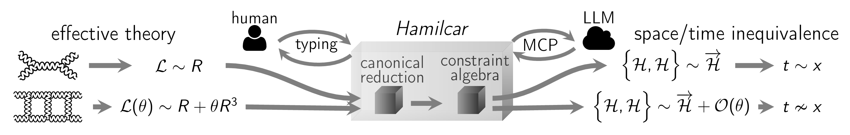
Hamiltonian (canonical) analysis toolkit for xAct
Version 0.0.0-developer
- Admits arbitrary tensorial field theories in 3+1 dimensions.
- Admits field theory on flat spacetime, or a dynamical metric for gravity.
- Keeps track of canonical fields and their conjugate momenta.
- Computes Poisson brackets between canonical quantities.
- Re-expresses computed brackets in terms of index-free ansätze using integrations by parts and dimensionally dependent identities.
- Can be used by humans.
- Can be used by agents.
License
Copyright © 2023 Will E. V. Barker
Hamilcar is distributed as free software under the GNU General Public License (GPL).
Hamilcar is provided without warranty, or the implied warranty of merchantibility or fitness for a particular purpose.
If Hamilcar was useful to your research, please cite us using the following BibTeX:
@article{Barker:2025noc,
    author = "Barker, Will",
    title = "{Fast Poisson brackets and constraint algebras in canonical gravity}",
    eprint = "2512.25007",
    archivePrefix = "arXiv",
    primaryClass = "physics.comp-ph",
    month = "12",
    year = "2025"
}
About
Hamilcar is a software package for Wolfram (formerly Mathematica) designed to provide robust tools for agentic systems to perform Hamiltonian analysis in canonical field theory. The overall goal is to enable AI agents and automated systems to conduct sophisticated field theory calculations through well-defined interfaces.
The package focuses on canonical field theory calculations in 3+1 dimensions, where the action $S$ has the structure
S=\int\mathrm{d}t\int\mathrm{d}^3x\ \Big[\pi_\psi(x,t)\cdot\dot{\psi}(x,t)-H(\psi,\pi_\psi)\Big],
where the ingredients are:
- The dynamical fields $\psi(x,t)$ are real tensors on the spatial manifold, which may be a collection of distinct fields, each field having some collection of spatial indices ($a$, $b$, etc.), perhaps with some symmetry among the indices.
- The conjugate momenta $\pi_\psi(x,t)$ are the canonical momenta conjugate to the fields $\psi(x,t)$.
- The Hamiltonian density $H(\psi,\pi_\psi)$ is constructed from the fields, momenta, spatial metric, and spatial derivatives.
Example: scalar field theory
As a demonstration, we consider a simple scalar field theory in 3+1 dimensions
S=\int\mathrm{d}^4x\ \Big[-\tfrac{1}{2}\partial^\mu\phi\partial_\mu\phi+\tfrac{1}{2}m^2\phi^2\Big],
where $m$ is the mass parameter.
In a fresh notebook we first load the package:
<<xAct`Hamilcar`;
Next, we define a scalar field using the command DefCanonicalField:
DefCanonicalField[Phi[],FieldSymbol->"\[Phi]",MomentumSymbol->"\[Pi]"];
We can then compute Poisson brackets between quantities:
PoissonBracket[Phi[],ConjugateMomentumPhi[]];
Documentation
Documentation with general relativity as a worked example is available at xAct/Hamilcar/Documentation/English/. Currently, the documentation is programmatically generated from the Documentation.m script, which uses some custom packages to produce Documentation.nb and Documentation.pdf files. The notebook and PDF are readable, and display the relevant commands in code blocks, however the notebook is not meant to be interactive or executable. More standard documentation may be added in future releases. It is also recommended to read the associated paper (see top of this README).
Agentic Integration
While Hamilcar currently provides a comprehensive Mathematica interface for canonical field theory calculations, it is intended for integration with agentic systems. A rudimentary agent Hasdrubal is under development.
General use
Pre-defined geometry
When you first run <<xAct`Hamilcar` the software defines a three-dimensional spatial hypersurface with the ingredients:
| Wolfram Language | Output format | Meaning |
|---|---|---|
a, b, c, …, z |
$a$, $b$, $c$, … $z$ | Spatial coordinate indices (corresponding to adapted coordinates in the ADM prescription) |
G[-a,-b] |
$\gamma_{ab}$ | Induced metric on the spatial hypersurface |
CD[-a]@ |
$\mathcal{D}_{a}$ | Spatial covariant derivative |
epsilonG[-a,-b,-c] |
$\epsilon_{abc}$ | Induced totally antisymmetric tensor on the spatial hypersurface |
For those familiar with xAct, note that calls to DefManifold and DefMetric are made internally at this stage. The package establishes a spatial manifold M3, creating the necessary geometric structure for canonical field theory calculations.
Function DefCanonicalField
DefCanonicalField[<Fld>[]]
defines a scalar canonical field <Fld> and its conjugate momentum ConjugateMomentum<Fld>.
DefCanonicalField[<Fld>[<Ind1>,<Ind2>,...]]
defines a tensor canonical field <Fld> and its conjugate momentum ConjugateMomentum<Fld> with indices <Ind1>, <Ind2>, etc..
DefCanonicalField[<Fld>[<Ind1>,<Ind2>,...],<Symm>]
defines a tensor canonical field <Fld> and its conjugate momentum ConjugateMomentum<Fld> with indices <Ind1>, <Ind2>, etc. and symmetry <Symm>.
Details and options
- The syntax of
DefCanonicalFieldfollows similar patterns toDefTensorin xTensor. - Any number of comma-separated indices may be drawn from the contravariant
a,b,c, up toz, the covariant-a,-b,-c, up to-z, or any admixture. - The symmetry
<Symm>can be one of the following (or any admixture allowed byDefTensor):Symmetric[{<SymmInd1>,<SymInd2>,...}]denotes symmetrized indices.Antisymmetric[{<SymmInd1>,<SymInd2>,...}]denotes antisymmetrized indices.
- If the global variable
$DynamicalMetricis set toTrue, then:- The spatial metric
Gis automatically registered as a canonical field, andConjugateMomentumGis defined. - All conjugate momenta are automatically defined as tensor densities of weight one (the effects of this are only seen by the
G-variations performed internally byPoissonBracket).
- The spatial metric
- The following options may be given:
FieldSymbolis the symbol that<Fld>will use for display formatting.MomentumSymbolis the symbol that the conjugate momentum will use for display formatting.
Function PoissonBracket
PoissonBracket[<Op1>,<Op2>]
computes the Poisson bracket between operators <Op1> and <Op2>.
Details and options
- The operators
<Op1>and<Op2>must be expressions involving:- Canonical fields and their conjugate momenta which have been defined using
DefCanonicalField. - Tensors which have been defined on the manifold
M3usingDefTensor, and which are assumed always to be independent of the canonical fields. - Derivatives via
CDof canonical and non-canonical quantities, the spatial metricG, and the totally antisymmtric tensorepsilonG. - Constant symbols which have been defined using
DefConstantSymbol(orDefNiceConstantSymbolfrom the xTras package).
- Canonical fields and their conjugate momenta which have been defined using
- The function automatically generates smearing tensors unless
$ManualSmearingis set toTrue. - When
$DynamicalMetricis set toTrue, theG-sector contributions are included. - The function computes variational derivatives with respect to all registered fields and momenta.
Function TotalFrom
TotalFrom[<Expr>]
expands composite expressions to canonical variable form by applying all registered expansion rules.
Details and options
- The function converts composite quantities (like constraint expressions, traces, or field combinations) into explicit expressions involving only the fundamental canonical variables: fields, conjugate momenta, and their spatial derivatives.
- This expansion is essential before computing Poisson brackets, as bracket calculations require expressions to be written in terms of the canonical variables registered by
DefCanonicalField. - The function applies all rules stored in the internal list
$FromRulesTotal, which are populated usingPrependTotalFrom.
Function TotalTo
TotalTo[<Expr>]
converts expressions from canonical variable form back to compact notation using registered contraction rules.
Details and options
- The function performs the inverse operation of
TotalFrom, converting expressions written in terms of canonical variables back to more compact composite notation. - This is primarily used for presentation purposes to make final results more readable.
- The function applies all rules stored in the internal list
$ToRulesTotal, which are populated usingPrependTotalTo. - Unlike
TotalFrom, this function is optional in most calculations.
Function PrependTotalFrom
PrependTotalFrom[<Rule>]
registers an expansion rule to convert a composite quantity to canonical variable form.
Details and options
- The function adds
<Rule>to the front of the internal list$FromRulesTotalused byTotalFrom. - Typically used with
MakeRuleexpressions that define composite quantities in terms of canonical variables. - Essential for setting up the expansion system before performing Poisson bracket calculations.
- Example usage:
FromSuperHamiltonian//PrependTotalFromregisters the rule to expand the super-Hamiltonian constraint.
Function PrependTotalTo
PrependTotalTo[<Rule>]
registers a contraction rule to convert canonical variable expressions back to compact notation.
Details and options
- The function adds
<Rule>to the front of the internal list$ToRulesTotalused byTotalTo. - Used with rules that convert expanded canonical expressions back to composite quantities.
- Provides the symmetric counterpart to
PrependTotalFromfor bidirectional transformations. - Less commonly used than
PrependTotalFromas conversion back to compact form is often optional.
Function FindAlgebra
FindAlgebra[<Expr>,{{<Fctr1>,<Fctr2>,...},...}]
seeks to express <Expr> as a sum of any number of terms, where each term corresponds to one of the sub-lists and has factors corresponding to indexed tensors whose heads are <Fctr1>, <Fctr2>, etc., where those tensor heads were defined using DefCanonicalField or DefTensor. The re-expression is achieved automatically by means of any required number of integrations by parts.
FindAlgebra[<Expr>,{{<Fctr1>,<Fctr2>,...,{CD,...,<Fctr3>,...}},...}]
additionally admits terms where one or more applications of the spatial covariant derivative CD act on any of a select group of factors, here <Fctr3>, etc.
Details and options
- The following options may be given:
Constraintsis a list of special (and appropriately indexed) tensors which were passed as part of the ansatz, with respect to which the re-expression is expected to be homogeneously linear. The answer will be expressed with these tensors factored out.Verifyis a boolean which, when set toTrue, causes the re-expression and<Expr>to be varied internally with respect to any tensors which appear exactly to the first power in all terms, after an application ofTotalFrom. This usually includes smearing functions, but it may also include some canonical variables. The equality of the variations is checked to ensure that the re-expression is correct. Default isFalse.DDIsis a boolean which, when set toTrue, causes dimensionally dependent identities (DDIs) such as the Cayley-Hamilton theorem to be taken into account when performing the re-expression. Default isFalse.
Function TimeD
This function is undocumented and under active development. The purpose of the function is to manage time derivatives of fields.
Quickstart
Requirements
Basic hardware requirements
- A multi-core processor (recommended, note that most modern PCs are multi-core).
- An internet connection (recommended for Hamilcar to interrogate the Wolfram Function Repository).
Operating systems
- Linux (recommended, tested on Linux v 6.15.8 via Arch, Manjaro, RockyLinux 8 (RHEL8), CentOS7 (RHEL7)) and Ubuntu.
- macOS (not recommended, tested on macOS Monterey).
- Windows (not recommended, tested on Windows 10).
Software dependencies
- Wolfram (formerly Mathematica) (required, tested on Wolfram v 14.2.0.0).
- xAct (required packages xTensor, SymManipulator, xPerm, xCore and xTras, tested on xAct v 1.2.0).
Installation
:warning: Note that Mathematica was re-branded as Wolfram on July 31 2024 with the release of Wolfram v 14.1. You may still be able to install Hamilcar in older versions of Wolfram (formerly Mathematica) by replacing Wolfram with Mathematica in the various paths below.
Linux
- Prepare. Make sure your system satisfies all the requirements.
- Download. You can download the latest release from the panel on the right, and unzip using:
```console, bash
[user@system ~]$ unzip ~/Downloads/Hamilcar*
[user@system ~]$ mv ~/Hamilcar* ~/Hamilcar
Alternatively, if you have _git_ installed, the following _bash_ command will download _Hamilcar_ into the home directory: ```console, bash, git [user@system ~]$ git clone https://github.com/wevbarker/Hamilcar - Install. To perform the installation, the sources need only be copied to the location of the other xAct sources. For a global installation of xAct this may require:
```console, bash
[user@system ~]$ cd Hamilcar/xAct
[user@system xAct]$ sudo cp -r Hamilcar /usr/share/Wolfram/Applications/xAct/
For a local installation of _xAct_, the path may be vary:
```console, bash
[user@system xAct]$ cp -r Hamilcar ~/.Wolfram/Applications/xAct/
macOS
:warning: Note that macOS is not recommended for use with Hamilcar.
- Prepare. Make sure your system satisfies all the requirements.
- Download. You can download the latest release from the panel on the right, and unzip using:
```console, zsh
user@system ~ % unzip ~/Downloads/Hamilcar*
user@system ~ % mv ~/Hamilcar* ~/Hamilcar
Alternatively, if you have _git_ installed, the following _zsh_ command will download _Hamilcar_ into the home directory: ```console, zsh, git user@system ~ % git clone https://github.com/wevbarker/Hamilcar - Install. To perform the installation, the sources need only be copied to the location of the other xAct sources. For a global installation of xAct this may require:
```console, zsh
user@system ~ % cd Hamilcar/xAct
user@system xAct % sudo cp -r Hamilcar /Library/Mathematica/Applications/xAct/
For a local installation of _xAct_, the path may be vary:
```console, zsh
user@system xAct % cp -r Hamilcar ~/Library/Mathematica/Applications/xAct/
Microsoft Windows
:warning: Note that Microsoft Windows is not recommended for use with Hamilcar.
- Prepare. Make sure your system satisfies all the requirements.
- Download. You can download the latest release from the panel on the right, and unzip in File Explorer using right-click and Extract All. Alternatively, if you have git installed, the following cmd command will download Hamilcar into the home directory:
console, cmd, git C:\Users\user> git clone https://github.com/wevbarker/Hamilcar - Install. To perform the installation, the sources need only be copied to the location of the other xAct sources. For a global installation of xAct, you may need to open File Explorer using right-click and Run as administrator. Alternatively, use the following cmd commands (again, opening cmd using Run as administrator):
```console, cmd
C:\Users\user> cd Hamilcar
C:\Users\user\Hamilcar> xcopy /e /k /h /i xAct\ “C:\Program Files\Wolfram Research\Mathematica\14.0\AddOns\Applications\xAct"
For a local installation of _xAct_, the path may be vary:
```console, cmd
C:\Users\user\Hamilcar> xcopy /e /k /h /i xAct\ "C:\Users\user\AppData\Roaming\Mathematica\Applications\xAct\"
Getting help
There are several ways to get help:
- The xAct google group contains a well established, highly active and very friendly community of researchers. Feel free to start a New conversation by posting a minimal working example of your code.
- For private correspondence, you can email barker@fzu.cz.
- Alternatively you may wish to raise a New issue on GitHub.
Acknowledgements
Hamilcar was improved by useful discussions with Boris Bolliet, Justin Feng, Drazen Glavan, Will Handley, Carlo Marzo, Roberto Percacci, Syksy Rasanen, Alessandro Santoni, Ignacy Sawicki, Richard Woodard and Tom Zlosnik.
I am grateful for the support of Marie Sklodowska-Curie Actions and the Institute of Physics of the Czech Academy of Sciences.
I was supported by the research environment and infrastructure of the Handley Lab at the University of Cambridge.
This work was performed using the Cambridge Service for Data Driven Discovery (CSD3), part of which is operated by the University of Cambridge Research Computing on behalf of the STFC DiRAC HPC Facility (www.dirac.ac.uk). The DiRAC component of CSD3 was funded by BEIS capital funding via STFC capital grants ST/P002307/1 and ST/R002452/1 and STFC operations grant ST/R00689X/1. DiRAC is part of the National e-Infrastructure.
Co-funded by the European Union (Physics for Future - Grant Agreement No. 101081515). Views and opinions expressed are however those of the author(s) only and do not necessarily reflect those of the European Union or European Research Executive Agency. Neither the European Union nor the granting authority can be held responsible for them.
Hasdrubal
A multi-agent system for automating the Dirac-Bergmann algorithm in canonical field theory.
Overview
Hasdrubal orchestrates the complete Dirac-Bergmann Hamiltonian constraint analysis for free bosonic field theories, from start to finish, without user intervention. The system delegates Poisson bracket computations to Hamilcar via a Wolfram kernel, while using large language model inference for high-level algorithmic decisions.
You can find a write-up of the results here.
Requirements
- Python 3.9+
- Wolfram Mathematica (with valid license) or Wolfram Engine
- OpenAI API key with access to GPT-5.2
- Hamilcar package for xAct/Mathematica (installation instructions)
Installation
- Clone the repository:
git clone https://github.com/wevbarker/Hasdrubal.git cd Hasdrubal - Create and activate a virtual environment:
python -m venv venv source venv/bin/activate - Install dependencies:
pip install -r requirements.txtKey dependencies include:
openai-agents(0.6.3) - OpenAI Agents SDKwolframclient(1.4.0) - Wolfram kernel interfacetenacity(9.1.2) - Retry logic for rate limitsmcp(1.18.0) - Model Context Protocol
- Install Hamilcar in Mathematica (see Hamilcar README).
Configuration
Create config/.env with your OpenAI API key:
cp config/.env.example config/.env
# Edit config/.env with your API key
The configuration file should contain:
OPENAI_API_KEY=sk-proj-your-key-here
The API key must have access to GPT-5.2. Configuration in config/.env takes precedence over environment variables.
Usage
Activate the virtual environment and run the REPL:
source venv/bin/activate
python hasdrubal_repl/hasdrubal_repl.py [OPTIONS]
Options
| Flag | Description |
|---|---|
-f FILE |
Load initial prompt from a markdown file |
-a |
Auto mode: automatically confirms each step |
Examples
Interactive mode (manual confirmation at each step):
python hasdrubal_repl/hasdrubal_repl.py -f hasdrubal_tests/ProcaTheory.md
Autonomous mode (full autopilot):
python hasdrubal_repl/hasdrubal_repl.py -f hasdrubal_tests/ProcaTheory.md -a
In autonomous mode, the agent runs until it issues TERMINATE, then provides a summary and returns control to the user.
Reproducing Paper Results
The sessions/ directory contains the actual session logs from the paper. The hasdrubal_tests/ directory contains input templates for running new analyses.
Paper Examples
| Paper Section | Theory | Input File | Paper Session ID |
|---|---|---|---|
| II.C | Massive longitudinal vector | ProcaTheory.md |
af268283-... |
| II.C | Massless longitudinal vector | MaxwellTheory.md |
0a434ed6-... |
| II.C | Massive multi-particle | CombinedTheory1.md |
526d8477-... |
| II.C | Massless multi-gauge | CombinedTheory2.md |
75456557-... |
| II.C | Li-Gao theory | ZlosnikTheory.md |
106ddac7-... |
Running an Example
To reproduce the Li-Gao theory analysis:
python hasdrubal_repl/hasdrubal_repl.py -f hasdrubal_tests/ZlosnikTheory.md -a
Note that input files use obfuscated variable names (hashes) to prevent the model from recognizing specific theories from its training corpus. Each run generates a new session with fresh obfuscation.
Session Logs
Sessions are stored as JSONL files in sessions/, with each line containing:
{"timestamp": "2025-12-18T00:04:13.424450Z", "type": "user", "content": "..."}
{"timestamp": "2025-12-18T00:04:21.985390Z", "type": "assistant", "content": "..."}
The type field indicates the message source:
user- User input (including auto-injected prompts and challenges)assistant- Agent responseserror- Error messages
Session filenames are UUIDs (e.g., 106ddac7-697f-4f87-a871-c98ebdd1829a.jsonl).
Architecture
Hasdrubal is a heterogeneous multi-agent system with two components:
-
LLM Agent (
hasdrubal_agent/) - Orchestrates the Dirac-Bergmann algorithm using GPT-5.2 via the OpenAI Agents SDK. The system prompt includes Hamilcar sources and worked examples for in-context learning. -
REPL Agent (
hasdrubal_repl/) - Regulates the LLM agent via yes/no responses, challenges, and error recovery. Implemented with regex and a fixed decision tree.
The agents communicate via the Model Context Protocol (MCP). The MCP server (hasdrubal_agent/mcp_server.py) exposes tool_WolframScript for executing arbitrary Wolfram Language code in a persistent Hamilcar kernel.
See Section II of the paper for full architectural details.
License
MIT License. See LICENSE for details.
:warning: As of January 2026, HiGGS has been deprecated by Hamilcar and is no longer actively maintained.

![]()
![]()
![]()
Hamiltonian Gauge Gravity Surveyor (HiGGS)
Version 1.2.3
- Feature: abstract indices representing gauge-fixed theory given cleaner formatting with Gothic script, extended indices
a1,b1,c1etc. denoted by primes. - Feature: provide more intuitive formatting of Poisson brackets in terms of smearing functions, as seen in output of
PoissonBracketandViewTheory. - Patch: fix shadowing error messages during the
NeedsorGetpackage call preamble. - Patch: fix Issue #1, loading of binaries on Windows.
- Patch: fix errors produced by
PoissonBracketwith the option"Surficial"->True. This error follows from sign errors in line two of Equation (E3) in 2205.13534, and generates nonphysical surface terms. My particular thanks to Manuel Hohmann for identifying this.
License
Copyright © 2022 Will E. V. Barker
HiGGS is distributed as free software under the GNU General Public License (GPL).
HiGGS is provided without warranty, or the implied warranty of merchantibility or fitness for a particular purpose.
Users of HiGGS, including authors of derivative works as defined by the GPL, are kindly requested to cite the 2022 HiGGS papers (2206.00658 and 2205.13534) in their resulting publications.
These conditions apply to all software in this repository, including “HPC-EEG” visualisation tools.
About
HiGGS is an (unofficial) part of the xAct bundle. It provides tools for the Hamiltonian constraint analysis (canoncical analysis or Dirac-Bergmann algorithm) of gravity with spacetime curvature and torsion. HiGGS can be used on a desktop PC, but it is parallelised for theory surveys on clusters and supercomputers.
Installation
Requirements
HiGGS has been tested in the following environment(s):
- Linux x86 (64-bit), specifically Manjaro, Arch, CentOS, Scientific Linux and Ubuntu
- Windows 10, as of HiGGS v 1.2.3
- Mathematica v 11.3.0.0
- xAct v 1.2.0
Install
- Make sure you have installed xAct.
- Download HiGGS:
bash, git git clone https://github.com/wevbarker/HiGGS cd HiGGS - Place the
./xAct/HiGGSdirectory relative to your xAct install. A global install might have ended up at:/usr/share/Mathematica/Applications/xActQuickstart
The package loads just like any other part of xAct, just open a fresh notebook and run:
Needs["xAct`HiGGS`"];
This loads the package (i.e. the names of the functions provided), along with its dependencies in the xAct bundle. However it does not load the physics. To construct the HiGGS environment, one must run:
BuildHiGGS[];
The build process may take about a minute or so. When it has concluded, you should be able to proceed to science. For example, try evaluating the Poisson bracket between the spin-parity 2+ irreducible component of the foliation-projected momentum of the translational gauge field, and the 1- irrep of the foliation-projected torsion tensor, without first defining a constraint shell for a particular theory, type:
PoissonBracket[PiPB2p[-a, -b], TP1m[-c], "ToShell" -> False];
If you want to try something more ambitious, build the constraint structure for Einstein-Cartan theory:
DefTheory[{Alp1 == 0, Alp2 == 0, Alp3 == 0, Alp4 == 0, Alp5 == 0,
   Alp6 == 0, Bet1 == 0, Bet2 == 0, Bet3 == 0, cAlp1 == 0, cAlp2 == 0,
    cAlp3 == 0, cAlp4 == 0, cAlp5 == 0, cAlp6 == 0, cBet1 == 0,
   cBet2 == 0, cBet3 == 0}, "Export" -> "EinsteinCartan"];
That output is less easy to show.
Installation test
More general examples can be found in the notebook ./xAct/HiGGS/Documentation/Examples/tutor.nb. This notebook also acts as an install test.
- Move the test files into your working directory, e.g. for a global install:
cp /usr/share/Mathematica/Applications/xAct/HiGGS/Documentation/Examples/tutor.nb ./ cp -r /usr/share/Mathematica/Applications/xAct/HiGGS/Documentation/Examples/svy ./ mkdir ./fig - Open Mathematica and run
./tutor.nbin a notebook front end. Make sure you run all the initialisation cells, from the beginning, to the end.
What’s in the box?
The HiGGS package has the following structure:
xAct
└── HiGGS
    ├── bin
    │   └── build
    │       ├── CanonicalPhiToggle.mx
    │       ├── CDPiPToCDPiPO3.mx
    │       ├── ChiPerpToggle.mx
    │       ├── ChiSingToggle.mx
    │       ├── CompleteO3ProjectionsToggle.mx
    │       ├── GeneralComplementsToggle.mx
    │       ├── NesterFormIfConstraints.mx
    │       ├── NonCanonicalPhiToggle.mx
    │       ├── O13ProjectionsToggle.mx
    │       ├── ProjectionNormalisationsToggle.mx
    │       └── VelocityToggle.mx
    ├── COPYING
    ├── Documentation
    │   ├── Examples
    │   │   ├── appcg.job.m
    │   │   ├── appcg.job.nb
    │   │   ├── appcg.job.sh
    │   │   ├── appcg.plt.py
    │   │   ├── appcg.plt.sh
    │   │   ├── peta4.job.m
    │   │   ├── peta4.job.nb
    │   │   ├── peta4.job.sh
    │   │   ├── peta4.job.slm
    │   │   ├── peta4.plt.py
    │   │   ├── peta4.plt.sh
    │   │   ├── peta4.rdm.png
    │   │   ├── peta4.svy.m
    │   │   ├── peta4.svy.nb
    │   │   ├── svy
    │   │   │   ├── EinsteinCartan.thr.mx
    │   │   │   ├── EinsteinCartan_vel.thr.mx
    │   │   │   ├── simple_spin_1p.thr.mx
    │   │   │   └── simple_spin_1p_vel.thr.mx
    │   │   ├── tutor.nb
    │   │   └── tutor.png
    │   ├── HiGGS.pdf
    │   └── HiGGS_sources.pdf
    ├── HiGGS.m
    ├── HiGGS.nb
    ├── HiGGS_smearing_functions_global.m
    ├── HiGGS_smearing_functions.m
    ├── HiGGS_SO3.m
    ├── HiGGS_SO3.nb
    ├── HiGGS_sources.m
    ├── HiGGS_sources.nb
    ├── HiGGS_variations.m
    └── Kernel
        └── init.wl
The license is in COPYING.
The file init.wl is called when the package is invoked, and points to HiGGS.m, a small Wolfram language file and main package file sourced by the notebook HiGGS.nb.
When the HiGGS environment is actually built, HiGGS.m is actually running HiGGS_sources.m - the larger “physics package” sourced by HiGGS_source.nb.
During the course of the build, the binaries ./xAct/HiGGS/bin/build/*.mx are incorporated; these contain some heavy expressions.
The sub-package HiGGS_variations.m incorporates elements of Cyril Pitrou’s code from this repository.
The files HiGGS.pdf and HiGGS_sources.pdf are carbon copies of the source notebooks.
The notebook tutor.nb contains some more basic examples, and it relies on the *.thr.mx files in the svy directory.
The Wolfram Language files which refer to smearing functions are patches in version 1.2.2.
What are peta4 and appcg?
The files ./xAct/HiGGS/Documentation/Examples/peta4.* and ./xAct/HiGGS/Documentation/Examples/appcg.* refer to the jobs which implement the HiGGS Commissioning Survey and various unit tests. HiGGS does not need these files to function. The names refer to two computing services:
- Peta-4 is a supercomputer, the CPU component of the heterogeneous CSD3 facility belonging to the University of Cambridge.
- appcg is a small, private compute server belonging to the Cavendish Laboratory Astrophysics Group.
These sources are included to give inspiration to users who which to perform HPC surveys, though the user’s architecture may well differ.
Contribute
Please do! I’m always responsive to emails (about science), so be sure to reach out at wb263@cam.ac.uk. I will also do my best to get your code working if you are just trying to use HiGGS.
Acknowledgements
This work was performed using resources provided by the Cambridge Service for Data Driven Discovery (CSD3) operated by the University of Cambridge Research Computing Service (www.csd3.cam.ac.uk), provided by Dell EMC and Intel using Tier-2 funding from the Engineering and Physical Sciences Research Council (capital grant EP/T022159/1), and DiRAC funding from the Science and Technology Facilities Council (www.dirac.ac.uk).
I am grateful for the kind hospitality of Leiden University and the Lorentz Institute, and am supported by Girton College, Cambridge.

![]()
![]()
xPlain: Formatting for Mathematical Derivations in Theoretical Physics
Version 0.0.0-developer
License
Copyright © 2023 Will E. V. Barker and Sebastian Zell
xPlain is distributed as free software under the GNU General Public License (GPL).
xPlain is provided without warranty, or the implied warranty of merchantibility or fitness for a particular purpose.
If xPlain was useful to your research, please cite us using the following BibTeX:
@misc{Barker:2023xPlain,
    author = "Barker, Will E. V. and Zell, Sebastian",
    title = "{xPlain: Formatting for Mathematical Derivations in Theoretical Physics}",
    year = "2023",
    note = "Part of the xAct bundle"
}
About
xPlain is a software package for Wolfram (formerly Mathematica) designed to format mathematical derivations in theoretical physics. It bridges the gap between programmatic computation and professional presentation by enabling both command-line and notebook interfaces while maintaining consistent, paper-quality mathematical typesetting.
The package addresses a fundamental challenge in theoretical physics: how to simultaneously:
- Retain the notebook front-end’s mathematical formatting capabilities
- Present calculations with paper-style layout
- Work entirely in plaintext using professional development tools
xPlain is an (unofficial) part of the xAct bundle and implements the FAIR guiding principles for scientific data management. It is designed for unambiguous, lasting derivations in the Wolfram Language and is suitable for researchers who use the Wolfram Language programmatically.
The package has been successfully used in published supplemental materials, receiving positive feedback from anonymous referees: “It is remarkable the effort made by the authors with the Supplemental Material to show the connection between the Mathematica code employed for the computations and the statements in the paper.”
Example: Basic Mathematical Document
As a demonstration, we consider formatting a simple mathematical derivation with sectioning, commentary, and cross-references.
In a fresh notebook we first load the package:
<<xAct`xPlain`;
Next, we create document structure using sectioning commands:
Title@"Welcome to the xPlain package, here is a title";
Chapter@"And here is a chapter";
Section@"And here is a section";
Subsection@"And here is a subsection";
We add commentary and define formatted variables:
Comment@"This is a comment. We will next type a numbered expression.";
Format@xx^=ToExpression@"\[ScriptX]";
DisplayExpression[xx,EqnLabel->"Eq1"];
For expressions that vanish, use the equation environment:
Comment@"And next we will type a numbered equation.";
DisplayEquation[xx,EqnLabel->"Eq2"];
Cross-references are handled automatically:
Comment@{"Here is a comment referring to",Cref@"Eq1",". We can also refer to multiple equations as",Cref@{"Eq1","Eq2"},"."};
Supercomment@{"Here is a comment referring to",Cref@"Eq1"," and multiple equations as",Cref@{"Eq1","Eq2"},"."};
The output is shown below:
Documentation
The package includes a comprehensive example notebook demonstrating all basic functionality. To run the examples:
[user@system xPlain]$ cp xAct/xPlain/Documentation/English/Examples.nb ~/Examples.nb
[user@system xPlain]$ cd ~
[user@system ~]$ wolframnb Examples.nb &
General use
Document Structure
The package provides hierarchical sectioning commands:
Title["title text"]- Document titleChapter["chapter text"]- Chapter headingSection["section text"]- Section headingSubsection["subsection text"]- Subsection heading
Commentary and Display
Comment["text"]orComment[{"text", Cref["label"], "more text"}]- Regular commentary with optional cross-referencesSupercomment[...]- Emphasized commentaryDisplayExpression[expr, EqnLabel->"label"]- Numbered mathematical expressionDisplayEquation[expr, EqnLabel->"label"]- Numbered equation (implies vanishing)
Cross-referencing
Cref["label"]- Reference to a single equationCref[{"label1", "label2"}]- Reference to multiple equationsMref["label"]- Alternative reference format
Mathematical Formatting
Format variables using standard Wolfram Language conventions:
Format@myvar^=ToExpression@"\[ScriptM]";
Quickstart
Requirements
Basic hardware requirements
- A multi-core processor (recommended)
- An internet connection (recommended for package dependencies)
Operating systems
- Linux (recommended, tested on Linux v 6.15.8 via Arch and Manjaro)
- macOS (tested on macOS Monterey)
- Windows (tested on Windows 10)
Software dependencies
- Wolfram (formerly Mathematica) (required, tested on Wolfram v 13.1.0.0)
- xAct (required, tested on xAct v 1.2.0)
Installation
:warning: Note that Mathematica was re-branded as Wolfram on July 31 2024 with the release of Wolfram v 14.1. You may still be able to install xPlain in older versions by replacing Wolfram with Mathematica in the paths below.
Linux
- Prepare. Make sure your system satisfies all the requirements.
- Download. Clone or download the repository:
[user@system ~]$ git clone https://github.com/wevbarker/xPlain - Install. Use the provided installation script:
[user@system xPlain]$ ./install.shAlternatively, manually copy to your xAct installation:
[user@system xPlain]$ cp -r xAct/xPlain ~/.Wolfram/Applications/xAct/For a global installation:
[user@system xPlain]$ sudo cp -r xAct/xPlain /usr/share/Wolfram/Applications/xAct/
macOS
- Prepare. Make sure your system satisfies all the requirements.
- Download. Clone or download the repository:
user@system ~ % git clone https://github.com/wevbarker/xPlain - Install. Copy to your xAct installation:
user@system xPlain % cp -r xAct/xPlain ~/Library/Mathematica/Applications/xAct/For a global installation:
user@system xPlain % sudo cp -r xAct/xPlain /Library/Mathematica/Applications/xAct/
Microsoft Windows
- Prepare. Make sure your system satisfies all the requirements.
- Download. Clone or download the repository:
C:\Users\user> git clone https://github.com/wevbarker/xPlain - Install. Copy to your xAct installation:
C:\Users\user\xPlain> xcopy /e /k /h /i xAct\ "C:\Users\user\AppData\Roaming\Mathematica\Applications\xAct\"For a global installation (run as administrator):
C:\Users\user\xPlain> xcopy /e /k /h /i xAct\ "C:\Program Files\Wolfram Research\Mathematica\14.0\AddOns\Applications\xAct\"
Getting help
There are several ways to get help:
- The xAct google group contains a well-established, highly active and very friendly community of researchers. Feel free to start a New conversation by posting a minimal working example of your code.
- For private correspondence, you can email us at wb263@cam.ac.uk.
- You may wish to raise a New issue on GitHub.
Acknowledgements
This work was performed using resources provided by the Cambridge Service for Data Driven Discovery (CSD3) operated by the University of Cambridge Research Computing Service (www.csd3.cam.ac.uk), provided by Dell EMC and Intel using Tier-2 funding from the Engineering and Physical Sciences Research Council (capital grant EP/T022159/1), and DiRAC funding from the Science and Technology Facilities Council (www.dirac.ac.uk).
I am grateful for the kind hospitality of Leiden University and the Lorentz Institute, and am supported by Girton College, Cambridge.

![]()
NoMoreNotebooks: Programmatic Wolfram Notebook Interface
Version 14.2
- Updated for Wolfram Language 14.2 compatibility
- Added support for both Wolfram and Mathematica FrontEnd commands
- Enhanced non-interactive mode for batch processing
License
Copyright © 2024 Will Barker
NoMoreNotebooks is distributed as free software under the GNU General Public License (GPL).
NoMoreNotebooks is provided without warranty, or the implied warranty of merchantibility or fitness for a particular purpose.
If NoMoreNotebooks was useful to your research, please consider citing this work.
About
NoMoreNotebooks is a software package for Wolfram (formerly Mathematica) designed to provide a programmatic interface to Wolfram notebooks. It enables running Wolfram Language code through a FrontEnd connection while maintaining complete control over notebook creation, evaluation, and output generation.
The package allows you to:
- Create and manipulate notebooks programmatically
- Execute Wolfram Language files in notebook environments
- Export notebook contents to various formats
- Control evaluation flow and timing
- Work in both interactive and batch processing modes
Example: Basic workflow
In a fresh notebook or kernel session, load the package:
<<NoMoreNotebooks`;
Establish a FrontEnd connection and create a target notebook:
Ignite[]
Load and execute a Wolfram Language file in the notebook:
Burn["myfile.m"]
Export the notebook to a file:
Singe["output.pdf"]
Close the notebook when finished:
Douse[]
Core Functions
Ignite[]
Establishes a FrontEnd connection and creates a target notebook with dark theme styling. This must be called before any other operations.
Burn[filename]
Loads and executes a .m file in the target notebook. The file is evaluated and the results are displayed in the notebook. The corresponding .nb file is automatically saved.
Douse[]
Closes the target notebook and cleans up the FrontEnd connection.
Singe[filename]
Exports the current notebook contents to the specified file format (typically PDF).
Smother[]
Aborts the current evaluation in the target notebook.
VimJ[]
Navigation helper that moves to the next cell in the notebook.
Configuration Variables
The package behavior can be customized through several global variables:
$NonInteractive: Set toTruefor batch processing mode (default:False)$TargetKernelName: Kernel name for evaluation (default:"NoMoreNotebooks")$DeletePauseTime: Delay time for cell operations in seconds (default:10)
Quickstart
Requirements
Basic hardware requirements
- A multi-core processor (recommended for better performance)
- Sufficient memory for Wolfram Language operations
Operating systems
Software dependencies
- Wolfram (formerly Mathematica) (required, tested on Wolfram v 14.2.0.0)
Installation
:warning: Note that Mathematica was re-branded as Wolfram on July 31 2024 with the release of Wolfram v 14.1. The package automatically detects your version and uses the appropriate commands.
Installation via script
-
Download. Clone or download this repository to your local system.
-
Install. Run the provided installation script:
./install.sh
This will copy the package to both ~/.Wolfram/Applications/ and ~/.Mathematica/Applications/ directories, ensuring compatibility with both new and legacy installations.
Manual installation
Alternatively, you can manually copy the NoMoreNotebooks/ directory to your Wolfram Applications directory:
Linux/macOS:
cp -r NoMoreNotebooks ~/.Wolfram/Applications/
cp -r NoMoreNotebooks ~/.Mathematica/Applications/  # For legacy versions
Windows:
Copy the NoMoreNotebooks/ folder to:
C:\Users\[username]\AppData\Roaming\Mathematica\Applications\C:\Users\[username]\AppData\Roaming\Wolfram\Applications\
Version Compatibility
The package automatically adapts to your Wolfram Language version:
- Version ≤ 14.0: Uses
mathematicacommand for FrontEnd launch - Version > 14.0: Uses
wolframnbcommand for FrontEnd launch
Interactive vs Non-Interactive Modes
Interactive Mode (default):
- Provides user feedback and status messages
- Includes timing delays for cell operations
- Suitable for development and testing
Non-Interactive Mode ($NonInteractive = True):
- Optimized for batch processing
- Minimal output and faster execution
- Waits for file operations to complete automatically
Use Cases
NoMoreNotebooks is particularly useful for:
- Batch processing: Running multiple Wolfram Language files systematically
- Automated reporting: Generating formatted notebook outputs programmatically
- Testing and validation: Running code in controlled notebook environments
- Documentation generation: Creating formatted mathematical documents
- Educational tools: Automating notebook creation for teaching materials
Getting Help
If you encounter issues or have questions:
- Check the function documentation within Wolfram Language using
?FunctionName - Ensure your Wolfram installation is properly configured
- Verify that the FrontEnd can be launched from your system
- For bug reports, please include your Wolfram version and operating system details
Development Notes
- The package requires a functional Wolfram FrontEnd installation
- FrontEnd connection is essential for all notebook operations
- The package handles version differences automatically
- Dark theme styling is applied by default for better visibility
- File operations include automatic saving and cleanup
![]()

Martensite
Adversarial hardening for modern grantsmanship
Logos (this part was written by a human)
Grantsmanship - the process of securing grants - is changing due to AI. This is an unprecedented, irreversible and unavoidable process, occurring at a rate which exceeds the adaptive capacity of all institutions and most individuals. From the accelerationist perspective, it is necessary to lean in to emerging technologies and ensure that they serve to maximise scientific productivity. This is, moreover, a duty incumbent on all researchers, owing to the importance of public trust in the academic enterprise.
Within Europe, applications for prestigious funding opportunities have risen sharply since 2022. Applicants are using LLMs to craft and refine their proposals, and referees are using LLMs to evaluate them. A minority of both applicants and referees deny this, including a dwindling subset who are telling the truth. Considering only the tools that are available at the time of writing, academia will naturally saturate in a configuration where LLM-assisted grantsmanship is not only ubiquitous, but also acceptable, and even expected. It will be argued elsewhere that this will have several benefits, including but not limited to:
- The liberation of time which can be spent on research, constituting a better use of public money.
- Mitigation of disadvantages which are utterly irrelevant to caliber of the researcher, such as being a non-native English speaker.
- Improved signal-to-noise ratio in gauging the excellence of ideas, due to all proposals having - and being expected to have - flawless presentation.
- A general diminution of grantsmanship itself as a proxy metric, and a return to results-based evaluation: “Stop promising to do things. What did you publish with your last grant, and who cited you?”
Martensite is intended to bring this saturation point forwards in time. The source code should be cloned, forked, or used a prompt for those wishing to roll their own system. The name derives from the hard, strong crystalline phase of steel formed by rapid quenching.
martensite -a application.pdf -c call_dir -P "I have been tasked with reviewing this research proposal, which is slightly outside of my area of expertise. Can you carefully examine the call text, and read the proposal, and draft a review for me?" -o report.pdf
Takes your research proposal application.pdf and the public call texts downloaded to call_dir, and generates multiple referee reports in report.pdf. The prompt is sent to the most advanced flagship models from OpenAI, Anthropic, and Google. You will need to have funded API keys for at least one provider.
Quick Start
For confident super-users. If you’re less comfortable in the terminal, proceed step-by-step through Installation below.
# Install dependencies
pip install -r requirements.txt

# Run a review with inline prompt
martensite -a application.pdf -P "Review this carefully"

# Run with call documentation
martensite -a application.pdf -c CallTexts/ -P "Review against these criteria"

# Run with custom output location
martensite -a CV.pdf -P "Focus on research impact" -o cv_review.pdf
Installation
1. PATH Configuration
The PATH tells your terminal where to find commands. This step lets you type martensite from any directory instead of typing the full path to the program.
Add Martensite to your PATH using either method:
Option A: Direct export
This adds Martensite to your PATH permanently.
# Add this line to your ~/.bashrc or ~/.zshrc
export PATH="$PATH:/path/to/Martensite"

# Reload your shell configuration
source ~/.bashrc  # or source ~/.zshrc
Option B: Symbolic link
This creates a shortcut in a directory that’s already in your PATH.
ln -s /path/to/Martensite/martensite.sh ~/.local/bin/martensite
2. Dependencies
Martensite is written in Python and generates referee reports as PDF files. You’ll need to install some additional software packages.
Python dependencies:
These are Python libraries that Martensite uses to communicate with AI providers and process documents.
pip install -r requirements.txt
Report dependencies:
PDF generation requires pandoc (document converter), LaTeX (typesetting system), and PDF utilities.
Linux (Arch/Manjaro):
sudo pacman -S pandoc texlive-core texlive-latexextra poppler
Linux (Debian/Ubuntu):
sudo apt install pandoc texlive-xetex texlive-latex-extra poppler-utils
macOS:
brew install pandoc poppler
brew install --cask mactex  # Or: brew install texlive
3. API Keys
Martensite supports three LLM providers. You need at least one API key to run reviews.
What are API keys?
If you’ve used ChatGPT through a web browser, you’ve been using OpenAI’s consumer interface. API keys let Martensite access the same AI models programmatically, directly from your computer. Unlike the web interface with a monthly subscription, API access is pay-as-you-go: you add funds to your account and pay only for what you use (typically a few cents per review). You’ll need to create a developer account with at least one provider (OpenAI, Anthropic, or Google) and add payment information before generating API keys.
How Martensite finds your keys:
Martensite checks three locations in order: environment variables → OS keyring → config file. Choose whichever method is most convenient for you.
Option A: Environment variables (recommended)
export OPENAI_API_KEY="sk-..."
export ANTHROPIC_API_KEY="sk-ant-..."
export GOOGLE_API_KEY="..."
Option B: OS keyring
# Uses system Keychain (macOS) or Secret Service (Linux)
keyring set llm/openai default    # paste key when prompted
keyring set llm/anthropic default
keyring set llm/google default
Option C: Config file
Create ~/.config/llm-keys/config.toml (Linux) or ~/Library/Application Support/llm-keys/config.toml (macOS):
[openai]
api_key = "sk-..."

[anthropic]
api_key = "sk-ant-..."

[google]
api_key = "..."
Platform Support
- Linux: Fully supported (tested on Arch, Ubuntu, Debian)
- macOS: Fully supported (10.15+ recommended)
Usage
Basic Review
martensite -a StatementOfPurpose.pdf -P "Review this research proposal"
With Call Documentation
martensite -a proposal.pdf -c CallTexts/ -P "Evaluate against call criteria"
Custom Output Path
martensite -a CV.pdf -P "Focus on career progression" -o reviews/cv_review.pdf
Dry Run (Testing)
martensite -a proposal.pdf -P "Test prompt" -o test.pdf -d
Command-Line Options
-a, --application: Path to PDF application file (required)-p, --prompt: Path to text file containing review prompt-P, --prompt-string: Review prompt as inline string-c, --call-docs: Path to directory or PDF with call documentation-o, --output: Output path for generated PDF (default: martensite.pdf)-d, --dry-run: Skip API calls and generate dummy reviews for testing-h, --help: Show help message
Project Structure
Martensite/
├── martensite/              # Core Python package
│   ├── __init__.py
│   ├── key_discovery.py     # Secure API key management
│   ├── application_reviewer.py  # Multi-LLM orchestration
│   ├── martensite_handler.py    # CLI backend handler
│   └── extract_pdf_text.py # PDF text extraction utilities
├── tests/                   # Test suite
│   ├── LaCaixaIASTRO/      # Test application files
│   └── *.sh                # Test scripts
├── martensite.sh           # Main CLI entry point
├── requirements.txt        # Python dependencies
└── README.md               # This file
Core Components
1. Multi-LLM Orchestration (application_reviewer.py)
- Parallel API calls across OpenAI, Anthropic, and Google models
- Configurable model selection for diverse perspectives
- PDF processing with text extraction
- Async execution for maximum performance
- Comprehensive error handling and retry logic
2. Secure Key Management (key_discovery.py)
- Environment variables checked first
- System keyring integration (keyctl/Keychain)
- XDG config directory fallback (~/.config/martensite/)
- Multi-provider support for OpenAI, Anthropic, Google
3. CLI Handler (martensite_handler.py)
- Argument parsing and validation
- PDF text extraction using PyPDF2
- Markdown generation with structured output
- PDF conversion via pandoc/XeLaTeX
- Token usage reporting
Supported Models
OpenAI
- GPT-5: Most advanced reasoning model
- GPT-4o: Flagship multimodal model
- o4-mini-2025-04-16: Cost-effective reasoning model
Anthropic
- claude-sonnet-4-5-20250929: Latest flagship model
- gemini-2.5-pro: Advanced multimodal model
Troubleshooting
“Command not found”: Check your PATH or use full path to martensite.sh
PDF extraction fails: Install PyPDF2 (pip install PyPDF2)
PDF conversion fails:
- Linux:
sudo apt install pandoc texlive-xetexorsudo pacman -S pandoc texlive-core - macOS:
brew install pandocandbrew install --cask mactex
Unicode errors: Ensure XeLaTeX is installed with Unicode font support
API key not found:
- Set environment variables:
export OPENAI_API_KEY=sk-... - Or use OS keyring:
keyring set llm/openai default(then paste key) - Or create config file:
- Linux:
~/.config/llm-keys/config.toml - macOS:
~/Library/Application Support/llm-keys/config.toml
- Linux:
Model fails: Check API call log in output for specific error messages
macOS: “Operation not permitted”: Grant Terminal full disk access in System Preferences → Security & Privacy
License
See LICENSE file for details.
Acknowledgements
I am indebted to Will Handley for (i) calling out zero-sum famine mentality on my part, and encouraging me to make this repository public, and (ii) funding the OpenAI inference used during development. I am also grateful to Ilona Gottwaldová for bringing the big picture of LLM-assisted grantsmanship to my attention.
![]()

Sauron
AI-powered academic collaborator discovery for theoretical physics
AI-powered academic collaborator discovery and ranking system using INSPIRE-HEP, GPT-4o web search, and Gemini 2.5 Pro.
Setup
Prerequisites:
- Python 3.8+
- API keys as environment variables:
export OPENAI_API_KEY="sk-..." export GOOGLE_API_KEY="..." - System:
wget,tar
Find your INSPIRE BAI:
- Go to https://inspirehep.net and search your name
- Copy your BAI from your profile (format:
FirstName.MiddleInitial.LastName.1)
Usage
1. Initialize
python sauron.py init --bai YOUR.INSPIRE.BAI.1
This creates confidential/ and downloads your papers.
2. Add Application Materials
Copy your research/teaching statements to:
confidential/GatherContext.md
Then re-run init:
python sauron.py init --bai YOUR.INSPIRE.BAI.1
3. Rank Collaborators
python sauron.py rank "Institution Name"
Examples:
python sauron.py rank "Institute of Cosmology and Gravitation at Portsmouth"
python sauron.py rank "Perimeter Institute for Theoretical Physics"
python sauron.py rank "SISSA"
Limit researchers (if token budget tight):
python sauron.py rank "Institution" --max-researchers 50
4. View Results
Results saved to output/Institution_Name/:
researchers.md- All researchers foundranking_context.md- Full context sent to Geminiranking.md- Final rankings
How It Works
Discovery:
- GPT-4o searches institution website for faculty names
- Names matched to INSPIRE profiles
- INSPIRE affiliation data used to find additional current researchers
- Filtered to current affiliations only
Ranking:
- Downloads 30 recent papers per researcher (titles/abstracts)
- Combines with your context:
- 5 recent papers (full LaTeX)
- All your papers (abstracts)
- Application materials
- Gemini 2.5 Pro ranks by:
- Existing research overlap
- Future research direction alignment
- Collaboration potential
Token optimization: ~345k base + ~7k per researcher = fits ~90-100 researchers in 1M token limit
Structure
Sauron/
├── sauron.py              # Main script
├── src/                   # Source code (VCS-safe)
├── confidential/          # Personal data (gitignored)
│   ├── papers/            # Your arXiv downloads
│   ├── cache/             # Collaborator papers
│   ├── MyPapers_Abstracts.md
│   ├── GatherContext.md   # Your applications (you provide)
│   └── BaseContext.md     # Generated
└── output/                # Results (gitignored, auto-generated)
Yes, output/ is auto-generated when you run rank commands.
Troubleshooting
“OPENAI_API_KEY not set” - export OPENAI_API_KEY=...
“No Google API key” - export GOOGLE_API_KEY=...
Token limit exceeded - Use --max-researchers 50
No researchers found - Use full institution name with department
Cost
~$3-4 per institution analysis (90 researchers, Gemini 2.5 Pro pricing)
Privacy
No personal info hardcoded. All personal data in confidential/ (gitignored). API keys from environment only.
License
See LICENSE file for details.
Ethics
This tool is intended for professional academic networking and job market research. It should:
- Help early-career researchers identify compatible mentors and collaborators
- Reduce geographic and social barriers in academic networking
- Assist in targeted, thoughtful outreach (not spam)
It should not be used for:
- Mass unsolicited emails
- Circumventing normal academic channels
- Research evaluation or hiring decisions without human review
Responsible use means reading the papers, engaging thoughtfully, and respecting researchers’ time.
Acknowledgements
I am indebted to Will Handley for (i) calling out zero-sum famine mentality on my part, and encouraging me to make this repository public, and (ii) funding the OpenAI inference used during development. I am also grateful to Ilona Gottwaldová for bringing the big picture of LLM-assisted grantsmanship to my attention.